In this post, we will provide an example of machine learning regression algorithm using the multivariate linear regression in Python from scikit-learn library in Python. The example contains the following steps:

Step 1: Import libraries and load the data into the environment.

Step 2: Generate the features of the model that are related with some measure of volatility, price and volume. 

Step 3: Visualize the correlation between the features and target variable with scatterplots.

Step 4: Create the train and test dataset and fit the model using the linear regression algorithm. 

Step 5: Make predictions, obtain the performance of the model, and plot the results. 

Step 1: Import libraries and load the data into the environment.

We will first import the required libraries in our Python environment.

import pandas as pd 
from datetime import datetime
import numpy as np 
from sklearn.linear_model import LinearRegression
import matplotlib.pyplot as plt

We will work with SPY data between dates 2010-01-04 to 2015-12-07.

First we use the read_csv() method to load the csv file into the environment. Make sure to update the file path to your directory structure.

SPY_data = pd.read_csv("C:/Users/FT/Documents/MachineLearningCourse/SPY_regression.csv")
 
# Change the Date column from object to datetime object 
SPY_data["Date"] = pd.to_datetime(SPY_data["Date"])
 
# Preview the data
SPY_data.head(10)

The data has the following structure:

 Date              Open                       High               Low                Close               Volume           Adj Close
0 2015-12-07  2090.419922  2090.419922  2066.780029  2077.070068  4.043820e+09  2077.070068
1 2015-12-04  2051.239990  2093.840088  2051.239990  2091.689941  4.214910e+09  2091.689941
2 2015-12-03  2080.709961  2085.000000  2042.349976  2049.620117  4.306490e+09  2049.620117
3 2015-12-02  2101.709961  2104.270020  2077.110107  2079.510010  3.950640e+09  2079.510010
4 2015-12-01  2082.929932  2103.370117  2082.929932  2102.629883  3.712120e+09  2102.629883
5 2015-11-30  2090.949951  2093.810059  2080.409912  2080.409912  4.245030e+09  2080.409912
6 2015-11-27  2088.820068  2093.290039  2084.129883  2090.110107  1.466840e+09  2090.110107
7 2015-11-25  2089.300049  2093.000000  2086.300049  2088.870117  2.852940e+09  2088.870117
8 2015-11-24  2084.419922  2094.120117  2070.290039  2089.139893  3.884930e+09  2089.139893
9 2015-11-23  2089.409912  2095.610107  2081.389893  2086.590088  3.587980e+09  2086.590088

Let's now set the Date as index and reverse the order of the dataframe in order to have oldest values at top.

# Set Date as index
SPY_data.set_index('Date',inplace=True)
 
# Reverse the order of the dataframe in order to have oldest values at top
SPY_data.sort_values('Date',ascending=True)

Step 2: Generate features of the model

We will generate the following features of the model:

• High - Low percent change
• 5 periods Exponential Moving Average
• Standard deviation of the price over the past 5 days
• Daily volume percent change
• Average volume for the past 5 days
• Volume over close price ratio

SPY_data['High-Low_pct'] = (SPY_data['High'] - SPY_data['Low']).pct_change()
SPY_data['ewm_5'] = SPY_data["Close"].ewm(span=5).mean().shift(periods=1)
SPY_data['price_std_5'] = SPY_data["Close"].rolling(center=False,window= 30).std().shift(periods=1)
 
SPY_data['volume Change'] = SPY_data['Volume'].pct_change()
SPY_data['volume_avg_5'] = SPY_data["Volume"].rolling(center=False,window=5).mean().shift(periods=1)
SPY_data['volume Close'] = SPY_data["Volume"].rolling(center=False,window=5).std().shift(periods=1)

Step 3: Visualize the correlation between the features and target variable

Before training the dataset, we will make some plots to observe the correlations between the features and the target variable.

jet= plt.get_cmap('jet')
colors = iter(jet(np.linspace(0,1,10)))
 
def correlation(df,variables, n_rows, n_cols):
    fig = plt.figure(figsize=(8,6))
    #fig = plt.figure(figsize=(14,9))
    for i, var in enumerate(variables):
        ax = fig.add_subplot(n_rows,n_cols,i+1)
        asset = df.loc[:,var]
        ax.scatter(df["Adj Close"], asset, c = next(colors))
        ax.set_xlabel("Adj Close")
        ax.set_ylabel("{}".format(var))
        ax.set_title(var +" vs price")
    fig.tight_layout() 
    plt.show()
        
# Take the name of the last 6 columns of the SPY_data which are the model features
variables = SPY_data.columns[-6:]  
 
correlation(SPY_data,variables,3,3)

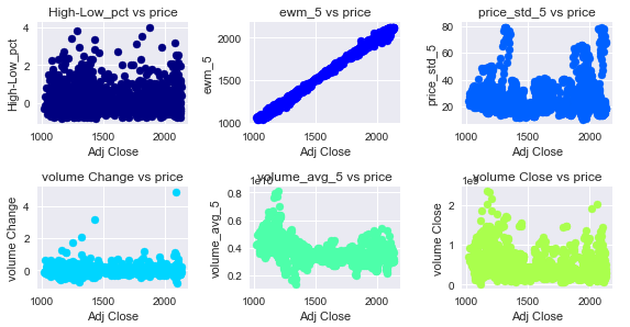
Correlations between Features and Target Variable (Adj Close)

The correlation matrix between the features and the target variable has the following values:

SPY_data.corr()['Adj Close'].loc[variables]

High-Low_pct         -0.010328
ewm_5                    0.998513
price_std_5              0.100524
volume Change       -0.005446
volume_avg_5        -0.485734
volume Close        -0.241898

Either the scatterplot or the correlation matrix reflects that the Exponential Moving Average for 5 periods is very highly correlated with the Adj Close variable. Secondly is possible to observe a negative correlation between Adj Close and the volume average for 5 days and with the volume to Close ratio.

Step 4: Train the Dataset and Fit the model

Due to the feature calculation, the SPY_data contains some NaN values that correspond to the first’s rows of the exponential and moving average columns. We will see how many Nan values there are in each column and then remove these rows.

SPY_data.isnull().sum().loc[variables]

High-Low_pct        1
ewm_5                   1
price_std_5             30
volume Change           1
volume_avg_5        5
volume Close        5

# To train the model is necessary to drop any missing value in the dataset.

SPY_data = SPY_data.dropna(axis=0)

# Generate the train and test sets

train = SPY_data[SPY_data.index < datetime(year=2015, month=1, day=1)]

test = SPY_data[SPY_data.index >= datetime(year=2015, month=1, day=1)]
dates = test.index

Step 5: Make predictions, obtain the performance of the model, and plot the results

In this step, we will fit the model with the LinearRegression classifier. We are trying to predict the Adj Close value of the Standard and Poor’s index. # So the target of the model is the "Adj Close" Column.

lr = LinearRegression()
 
X_train = train[["High-Low_pct","ewm_5","price_std_5","volume_avg_5","volume Change","volume Close"]]
 
Y_train = train["Adj Close"]
 
lr.fit(X_train,Y_train)      
 

Create the test features dataset (X_test) which will be used to make the predictions.

# Create the test features dataset (X_test) which will be used to make the predictions.

X_test = test[["High-Low_pct","ewm_5","price_std_5","volume_avg_5","volume Change","volume Close"]].values 

# The labels of the model

Y_test = test["Adj Close"].values 

Predict the Adj Close values using  the X_test dataframe and Compute the Mean Squared Error between the predictions and the real observations.

close_predictions = lr.predict(X_test)   

mae = sum(abs(close_predictions - test["Adj Close"].values)) / test.shape[0]

print(mae)

18.0904

We have that the Mean Absolute Error of the model is 18.0904. This metric is more intuitive than others such as the Mean Squared Error, in terms of how close the predictions were to the real price.

Finally we will plot the error term for the last 25 days of the test dataset. This allows observing how long is the error term in each of the days, and asses the performance of the model by date. 

# Create a dataframe that output the Date, the Actual and the predicted values
df = pd.DataFrame({'Date':dates,'Actual': Y_test, 'Predicted': close_predictions})
df1 = df.tail(25)
 
# set the date with string format for plotting
df1['Date'] = df1['Date'].dt.strftime('%Y-%m-%d')
 
df1.set_index('Date',inplace=True)
 
error = df1['Actual'] - df1['Predicted']
 
# Plot the error term between the actual and predicted values for the last 25 days
 
error.plot(kind='bar',figsize=(8,6))
plt.grid(which='major', linestyle='-', linewidth='0.5', color='green')
plt.grid(which='minor', linestyle=':', linewidth='0.5', color='black')
plt.xticks(rotation=45)
plt.show()

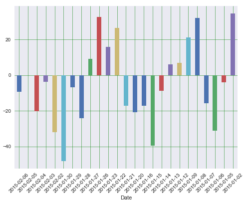
Error Term by date 

This concludes our example of Multivariate Linear Regression in Python.