Multiple Linear Regression

The multiple linear regression algorithm states that a response y can be estimated with a set of input features x and an error term ɛ. The model can be expressed with the following mathematical equation:

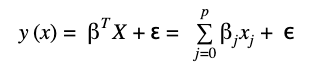
β^TX is the matrix notation of the equation, where β^T, X ϵ ʀ^p+1 and ɛ ~ N(μ,σ²)

β^T(transpose of β) and X are both real-valued vectors with dimension p+1 and ɛ is the residual term which represents the difference between the predictions of the model and the true observation of the variable y.

The vector β^T = (β₀,β₁,…β_P) stores all the beta coefficients of the model. These coefficients measure how a change on some of the independent variable impact on the dependent or target variable.

The vector X = (1,x₁,x₂, …x_p) hold all the values of the independent variables. Both vectors (T and X) are p+1 dimensional because of the need to include an intercept term.

The goal of the linear regression model is to minimize the difference between the predictions and the real observations of the target variable. For this purpose, a method called Ordinal Least Squares (OLS) is used which will derive the optimal set of coefficients for fitting the model.

Ordinal Least Squares

Formally the OLS model will minimize the Residual Sum of Squares (RSS) between the observations of the target variable and the predictions of the model. The RSS is the loss function metric to assess model performance in the linear regression model and has the following formulation:

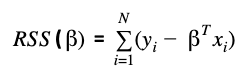
Residual Sum of Squares also known as the Sum of Squared Errors (SSE) between the predictions β^Tx_i and the observations y_i. With the minimization of this function, it is possible to get the optimal parameter estimation of the vector β.

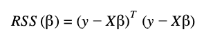
In matrix notation, the RSS equation is the following:

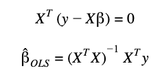
To get the optimal values of β, it is necessary to derivate RSS respect to β:

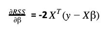
Remember that X is a matrix with all the independent variables and has N observations and p features. Therefore, the dimension of X is N (rows) x p+1 (columns).

One assumption of this model is that the matrix X^TX should be positive-define. This means that the model is valid only when there are more observations than dimensions. In cases of high-dimensional data (e.g. text document classification), this assumption is not true.

Under the assumption of a positive-definite X^TX the differentiated equation is set to zero and the β parameters are calculated:

Later we will show an example using a dataset of Open, High, Low, Close and Volume of the S&P 500 to fit and evaluate a multiple linear regression algorithm using Scikit learn library.

Series Navigation

‹ Supervised Learning ModelsLogistic Regression ›