Using the scikit-learn package from python, we can fit and evaluate a logistic regression algorithm with a few lines of code. Also, for binary classification problems the library provides interesting metrics to evaluate model performance such as the confusion matrix, Receiving Operating Curve (ROC) and the Area Under the Curve (AUC).

Hyperparameter Tuning in Logistic Regression in Python

In the Logistic Regression model (as well as in the rest of the models), we can change the default parameters from scikit-learn implementation, with the aim of avoiding model overfitting or to change any other default behavior of the algorithm. 

For the Logistic Regression some of the parameters that could be changed are the following:

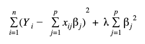
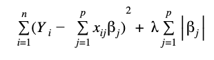
• Penalty: (string) specify the norm used for penalizing the model when its complexity increases, in order to avoid overfitting.  The possible parameters are “l1”, “l2” and “none”. “l1” is the Lasso Regression and “l2” is the Ridge Regression that represents two different ways to increase the magnitude of the loss function. Default value is “l2”. “none” means no regularization parameter. l1, lasso regression, adds “absolute value of magnitude” of coefficient as penalty term to the loss function. l2, ridge regression, adds “squared magnitude” of coefficient as penalty term to the loss function.
• C: (float): the default value is 1. With this parameter we manage the λ value of regularization as C = 1/λ.  Smaller values of C mean strong regularization as we penalize the model hard.
• multi_class: (string) the default value is “ovr” that will fit a binary problem. To fit a multiple classification should pass “multinomial”.
• solver: (string) algorithm to use in the optimization problem: “newton-cg”, “lbfgs”,”liblinear”,”sag”, and ”saga”. Default is “liblinear”. These algorithms are related to how the optimization problem achieves the global minimum in the loss function.
  • “liblinear”: is a good choice for small datasets
  • “Sag” or “saga”: useful for large datasets
  • “lbfgs”,”sag”,”saga”, or “newton-cg”: handle multinomial loss, so they are suitable for multinomial problems.
  • “liblinear” and “saga”: handle “l1” and “l2” penalty

The penalty has the objective to introduce regularization which is a method to penalize complexity in models with high amount of features by adding new terms to the loss function. 

It is possible to tune the model with the regularization parameter lambda (λ) and handle collinearity (high correlation among features), filter out noise and prevent overfitting. 

By increasing the value of lambda (λ) in the loss function we can control how well the model is fit to the training data. As stated above, the value of λ in the logistic regression algorithm of scikit learn is given by the value of the parameter C, which is 1/λ. 

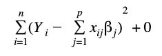
To show these concepts mathematically, we write the loss function without regularization and with the two ways of regularization: “l1” and “l2” where the term

are the predictions of the model.

Loss Function without regularization

Loss Function with l1 regularization

Loss Function with l2 regularization