Classifier Model in Machine Learning Using Python
In the post, we will learn about how to create a classifier model in machine learning using python. We will create a supervised classifier model that will train a dataset with a set of features and then use test data to predict price direction at day k with information only known at day k-1. Price direction can be up when the closing price at t is higher than the price at t-1, and down when the closing price at t is lower than at t-1.
For this task we create a set of features that are the lagged returns for the previous 2 days and volume percent change in each day. Then we train the dataset and fit different models with a set of algorithms that are the Logistic Regression, Support Vector Machine, Support Vector Classifier, Random Forest and Linear Discriminant Analysis.
For each of the model we will output two metrics that are used in classification problems to assess model performance. These metrics are the Hit Rate and the Confusion Matrix.
Hit Rate
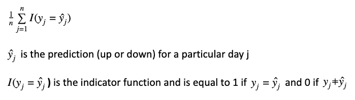
The Hit Rate provides a measure of the percentage of the number of times, the classifier make correct predictions (up and down). This indicator can be expressed with the following formula:
Confusion Matrix
The Confusion Matrix gives a measure of how many times the classifier predicts up correctly and how many times did predict down correctly.
In a binary classification problem, the confusion matrix is a 2 x 2 contingency table that determine the False Positive Rate (Type 1 error. When incorrectly reject a True null hypothesis. UF in the contingency table) and the False Negative Rate (Type II error. When fail to reject the null hypothesis. DF in the contingency table).
UT UF DF DT
UT represents correctly classify up periods, UF represents incorrectly classify up periods (they were classified as down periods), DF represents incorrectly classify down periods (they were classified us up periods), and DT represents correctly classify down periods.
Scikit Learn library provides methods to calculate the Hit Rate and the Confusion Matrix for a classifier. The dataset of the model is the SPY data between 2015-01-01 to 2019-09-18. We will load the dataset into the environment.
The python example below contains the following steps:
- Step 1: Import libraries, and load SPY data into the environment with the read_csv() function. This is the dataset of the model with dates between 2015-01-01 to 2019-09-18
- Step 2: Create features and target variable with the model_variables() function
- Step 3: Fit different models: Logistic Regression, Random Forest, Support Vector Machine, Linear Discriminant Analysis
- Step 4: Obtain metrics such as Confusion Matrix and Hit Rate for each of the models.
1import pandas as pd
2import numpy as np
3import datetime
4from sklearn.ensemble import RandomForestClassifier
5from sklearn.linear_model import LogisticRegression
6from sklearn.discriminant_analysis import LinearDiscriminantAnalysis as LDA
7from sklearn.metrics import confusion_matrix
8from sklearn.svm import LinearSVC, SVC
9data = pd.read_csv("C:/Users/Nicolas/Documents/Machine Learning Course/spy_data.csv",index_col='Date')
10
11def model_variables(prices,lags):
12    '''
13    Parameters:
14        prices: dataframe with historical data of SPY with the variables closes and
15        volume.
16        lags: Number of lags of the closing price that will be created by the function
17        to make the lagged returns features of the machine learning model
18    Output:
19        tsret: dataframe with index date, the independent variables(X) and the
20        dependent variable(y) of the machine learning model
21    '''
22
23    # Change data types of prices dataframe from object to numeric
24    prices = prices.apply(pd.to_numeric)
25    # Create the new lagged DataFrame
26    inputs = pd.DataFrame(index=prices.index)
27
28    inputs["Close"] = prices["Close"]
29    inputs["Volume"] = prices["Volume"]
30    # Create the shifted lag series of prior trading period close values
31    for i in range(0, lags):
32        tsret = pd.DataFrame(index=inputs.index)
33        inputs["Lag%s" % str(i+1)] = prices["Close"].shift(i+1)
34
35   #Create the returns DataFrame
36    tsret["VolumeChange"] =inputs["Volume"].pct_change()
37    tsret["returns"] = inputs["Close"].pct_change()*100.0
38
39    # If any of the values of percentage returns equal zero, set them to
40    # a small number (stops issues with QDA model in Scikit-Learn)
41    for i,x in enumerate(tsret["returns"]):
42        if (abs(x) < 0.0001):
43            tsret["returns"][i] = 0.0001
44
45    # Create the lagged percentage returns columns
46    for i in range(0, lags):
47        tsret["Lag%s" % str(i+1)] = \
48          inputs["Lag%s" % str(i+1)].pct_change()*100.0
49
50    # Create the "Direction" column (+1 or -1) indicating an up/down day
51    tsret = tsret.dropna()
52    tsret["Direction"] = np.sign(tsret["returns"])
53
54    # Convert index to datetime in order to filter the dataframe by dates when
55    # we create the train and test dataset
56    tsret.index = pd.to_datetime(tsret.index)
57    return tsret
58
59# Pass the dataset(data) and the number of lags 2 as the inputs of the model_variables  function
60variables_data = model_variables(data,2)
61
62# Use the prior two days of returns and the volume change as predictors
63# values, with direction as the response
64dataset = variables_data[["Lag1","Lag2","VolumeChange","Direction"]]
65dataset = dataset.dropna()
66
67# Create the dataset with independent variables (X) and dependent variable y
68X = dataset[["Lag1","Lag2","VolumeChange"]]
69y = dataset["Direction"]
70
71# Split the train and test dataset using the date in the date_split variable
72# This will create a train dataset of 4 years data and a test dataset for more than
73# 9 months data.
74
75date_split = datetime.datetime(2019,1,1)
76
77X_train = X[X.index <= date_split]
78X_test =  X[X.index > date_split]
79y_train = y[y.index <= date_split]
80y_test = y[y.index > date_split]
81
82# Create the (parametrised) models
83print("Hit Rates/Confusion Matrices:\n")
84models = [("LR", LogisticRegression()),
85              ("LDA", LDA()),
86              ("LSVC", LinearSVC()),
87              ("RSVM", SVC(
88                      C=1000000.0, cache_size=200, class_weight=None,
89                      coef0=0.0, degree=3, gamma=0.0001, kernel='rbf',
90                      max_iter=-1, probability=False, random_state=None,
91                      shrinking=True, tol=0.001, verbose=False)
92    ),
93    ("RF", RandomForestClassifier(
94            n_estimators=1000, criterion='gini',
95            max_depth=None, min_samples_split=2,
96            min_samples_leaf=30, max_features='auto',
97            bootstrap=True, oob_score=False, n_jobs=1,
98            random_state=None, verbose=0)
99    )]
100
101
102# Iterate through the models and obtain the accuracy metrix: Hit Rate and Consusion Matrix
103for m in models:
104    # Train each of the models on the training set
105    m[1].fit(X_train, y_train)
106    # Make an array of predictions on the test set
107    pred = m[1].predict(X_test)
108    # Output the hit-rate and the confusion matrix for each model
109
110    print("%s:\n%0.3f" % (m[0], m[1].score(X_test, y_test)))
111    print("%s\n" % confusion_matrix(pred, y_test))
112
The results of the code are the Hit Rate and the Confusion Matrix for each of the models trained. The diagonal of the matrix represent the correct predictions (up and down), and the inverse of the diagonal represents incorrect predictions (the prediction was down and the price go up, or the prediction was up and the price go down).
1LR:
20.583
3[[28 29]
4 [46 77]]
5
6LDA:
70.589
8[[28 28]
9 [46 78]]
10
11LSVC:
120.583
13[[28 29]
14 [46 77]]
15
16RSVM:
170.572
18[[20 23]
19 [54 83]]
20
21RF:
220.600
23[[34 32]
24 [40 74]]
25
The model with the best prediction score is the Random Forest with a Hit Rate of 60%. We have changed the default parameter min_samples_leaf of the Random Forest Classifier from it default value of 1 to 30.
This means that each leaf node has at least 30 observations and that a split will be considered if it leaves at least 30 training samples in each left and right branches. All the models work well to predict down periods respect up periods, as the true positive rate for the “down” days (DTDT+UF) is significantly higher than the true positive rate for the “up” days (UTUT+DF).
