The Support Vector Machine is a Supervised Machine Learning algorithm that can be used for both classification and regression problems. However, it is most used in classification problems. The goal of the algorithm is to classify new unseen objects into two separate groups based on their properties and a set of examples that are already classified. 

Some common applications for this algorithm are the following:

• Classify new documents into positive and negative sentiment categories based on other documents that have already been classified.
• Classify new emails into spam or not spam based on a large set of emails that have already been marked as spam or not spam.
• Bioinformatics (Protein Classification, Cancer Classification)
• Other tasks that are characterized to have a higher feature dimensional space.

The algorithm creates a partition of the features space into two subspaces. Once these subspaces are created, new unseen data can be classified in some of these locations. 

To address non-linear relationship, the algorithm follows a technique called the kernel trick to transform the data and find an optimal boundary between the possible outputs. Basically these are techniques to project the data into a higher dimension such that a linear separator would be sufficient to split the features space.

The separation between the two zones is given by a boundary which is called the hyperplane. Let us look at how the concept of hyperplane works in the Support Vector Machine algorithm.

Hyperplane

An interesting feature about the Support Vector Machine algorithm is that this hyperplane does not need to be a linear hyperplane. The hyperplane can introduce various types of non-linear decision boundaries. This feature increases the usability of the Support Vector Machine algorithm as it is capable to address non-linear relationships between features and target variables.

The algorithm will find the hyperplane that best separates the classes of the target variable by training a set of n observation of the features. Each observation is a pair of the p-dimensional vector of features (x1, x2, x3, …, xp) and the class yi which is the label. 

Usually the classes of the target variable are defined as +1 and -1, where each of these classes has their own meaning (negative vs positive, spam vs non-spam, malign vs benign). 

When yi = 1, it implies that the sample with the feature vector xi belongs to class 1 and if yi = −1, it implies that the sample belongs to class -1.

The +1 class could be “non-spam” or “positive” sentiment and the class -1 could be “spam” and “negative” sentiment.  Depending on which side of the hyperplane a new observation is located on, we assign it a particular class (-1, +1).

Deriving the hyperplane

The dimension of the hyperplane depends on the number of features. If the number of input features is two (R2), the hyperplane can be drawn as a line. If the number of input features is three, then the hyperplane becomes a two dimensional plane.

In order to optimize the hyperplane or the separation boundary between the two classes there are two important concepts that need to be described. These are the concepts of Maximal Margin Hyperplane (MMH) and the Maximal Margin Classifier (MMC).

Maximal Margin Hyperplane

The classes of a target variable can be well segregated by more than one hyperplane as we can observe in the figure below. However, we should select the hyperplane with the maximum distance between the nearest observations data points and the hyperplane, and this condition is achieved by the Maximal Margin Hyperplane.

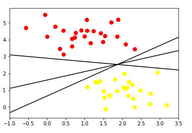
Multiples Separating Hyperplane

Therefore, maximizing the distance between the nearest points of each class and the hyperplane would result in an optimal separating hyperplane. 

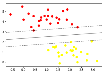
Maximum Separating Hyperplane

The continuous grey line in the above figure is the Maximal Margin hyperplane, as is the hyperplane that maximizes the distance between it and the nearest data points of the two classes. To find the Maximal Margin Hyperplane, it is necessary to compute the perpendicular distance from each of the training observations xi  for a given separating hyperplane.

The smallest perpendicular distance to a training observation from the hyperplane is known as the margin. The Maximum Margin Hyperplane is the separating hyperplane where the margin is the largest.

Non-linear relationships

Support Vector machine handles situations of non-linear relations in the data by using a kernel function which map the data into a higher dimensional space where a linear hyperplane can be used to separate classes.

If the data can’t be separated by linear discrimination, it is possible to use some trick to project the data in a higher dimension and apply a linear hyperplane. The figure below shows a scenario where the data cannot be separated using a linear hyperplane:

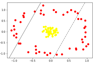
Non-linear separation to the data

In situations such as in this figure, Support Vector Machines algorithm becomes extremely powerful because using the kernel trick technique they can project the data into a higher-dimensional space and thereby we’re able to fit nonlinear relationships with a linear classifier.

Making a transformation of the space, and adding one more dimension to the data, will allow the data to be linearly separable. The following plot shows how the previous classes can be linearly separated with the increment of the dimension of the space from 2 dimensions to 3 dimensions. 

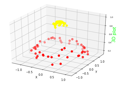
Kernel Transformation to 3D

The kernel trick represent a real strength in the Support Vector Machine algorithm as we can solve non-linear classification problems with efficiency. 

Support Vector Machine Python - Parameter Tuning

The Support Vector Machine  algorithm can be fit with the scikit learn library from python which provides a straightforward method to use this algorithm. It is possible to parametrize and tune important parameters of the algorithm that are explained below:

• Kernel: (string) select the type of hyperplane used to separate the data. The options are “linear”, “rbf”, “poly”. “linear” will use a linear hyperplane whereas “rbf” and “poly” uses a non-linear hyperplane. The default argument is “rbf”.
• Gamma:  (float) is a parameter for non-linear hyperplanes. The higher the gamma value more precisely it tries to fit the training data set. Default argument is “auto” which uses 1 / n_features. Low gamma value means to consider far away point when deciding the decision boundary.
• C: (float) is the penalty parameter of the error term. It regulates overfitting by controlling the trade-off between smooth decision boundary and classifying the training points correctly.  Greater values of C lead to overfitting to the training data.
• Degree: (integer) is a parameter used when kernel is set to “poly”. It is the degree of the polynomial used to find the hyperplane to split the data. The default value is 3. Using degree=1 is the same as using “linear” kernel.