Feature Selection is one of the core concepts in machine learning and has a high impact on the performance of the model. Irrelevant or partially irrelevant features can negatively impact the model performance.

In this process, those features which contribute most to the prediction variable are selected. In order to get an idea about which features could have more predictive power in a machine learning model, we will load Open, High, Low, Close, Volume (OHLCV) data for AMZ stock, and create some new features using Python.

Afterwards, we will use data visualizations and other common approaches for a smart selection of the features.

We will be performing this process using Python. The example below has 4 main steps:

• Import the Python libraries that will be used.
• Calculate Technical Indicators with the get_technical_indicators() function.
• Plot scatterplots among features and target variable _AdjClose._
• Make a Heat Map to show the correlation between each of the features and the target variable.
• Fit a Random Forest Model to extract feature importance of the independent variables (we will explain this algorithm in future sections but now will use some of the tools that Random Forest provides).

import pandas as pd
import matplotlib.pyplot as plt
import numpy as np
import seaborn as sns
from sklearn.ensemble import RandomForestRegressor

The data for AMZ stock is loaded into the environment using the read_csv() method.

# To read the file, make sure to provide path to the correct directory in your computer.

amz = pd.read_csv("C:/Users/Nicolas/Documents/Machine_Learning_Course/AMZ.csv")

We use the amz object dataframe which has OHLCV data from AMZ ticker and pass into the get_technical_indicators() function. This function generates technical indicators to be used as features for a machine learning model.

def get_technical_indicators(dataset):
    '''
    params:
        dataset: OHLCV data for AMZ ticker from 1999-09-01 to 2019-09-20
    returns    
        features dataframe with the calculations of all technical Indicators such as 
        MACD, 20 period’s standard deviation, ROC, CCI, EMA
    '''
    # Sort values by dates. Old dates at top 
    dataset.sort_index(inplace=True)
    # Create the features  dataframe to store only the features
    features = pd.DataFrame(index=dataset.index)
    
    # Create 7 and 21 days Moving Average
    features['ma7'] = dataset['AdjClose'].rolling(window=7).mean()
    features['ma21'] = dataset['AdjClose'].rolling(window=21).mean()
    
    # Create MACD
    features['26ema'] = dataset['AdjClose'].ewm(span=26).mean()
    features['12ema'] = dataset['AdjClose'].ewm(span=12).mean()
    features['MACD'] = (features['12ema']-features['26ema'])
 
    # Create Bollinger Bands
    features['20sd'] = dataset['AdjClose'].rolling(20).std()
    features['upper_band'] = features['ma21'] + (features['20sd']*2)
    features['lower_band'] = features['ma21'] - (features['20sd']*2)
    
    # Create Exponential moving average
    features['ema'] = dataset['AdjClose'].ewm(span=20).mean()
    
    # ROC Rate of Change
    N = dataset['AdjClose'].diff(10)
    D = dataset['AdjClose'].shift(10)
    features['ROC'] = N/D
    
    # CCI  Commodity Channel Index
    TP = (dataset['High'] + dataset['Low'] + dataset['AdjClose']) / 3 
    features['CCI']  = (TP - TP.rolling(20).mean()) / (0.015 *  TP.rolling(20).std() )
    # Create Average True Range 
    features['TR'] = dataset['High'] - dataset['Low']
    features['ATR'] = features['TR'].ewm(span = 10).mean()
 
    return features


# Store the output of get_technical_indicators() function in the features object

features = get_technical_indicators(amz)

The features object stores all the calculations of the get_technical_indicators() function.

# Retrieve the features that will be used  in the vars_ dataframe
vars_ = features[['MACD','20sd','TR','ma21','ROC','CCI']]
 
# The correlation() function would make scatterplots between each of the features and  the target variable AdjClose
 
jet= plt.get_cmap('jet')
colors = iter(jet(np.linspace(0,1,10)))
 
def correlation(df,features,variables, n_rows, n_cols):
    fig = plt.figure(figsize=(8,6))
    #fig = plt.figure(figsize=(14,9))
    for i, var in enumerate(variables):
        ax = fig.add_subplot(n_rows,n_cols,i+1)
        asset = features.loc[:,var]
        ax.scatter(df["AdjClose"], asset, c = next(colors))
        ax.set_xlabel("AdjClose")
        ax.set_ylabel("  {}".format(var))
        ax.set_title(var +" vs AdjClose")
    fig.tight_layout() 
    plt.show()
        
columns = vars_.columns    
correlation(amz,vars_,columns,2,3)

Figure 1: Feature Selection Scatterplots

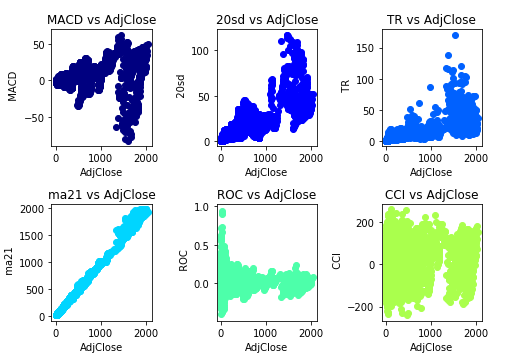
The scatterplot shows that there is an extremely positive correlation between the ma21 variable and the AdjClose. We can also visualize that there is a positive correlation between the 20sd and the TR variables with the target variable AdjClose. 

On the other hand, there is a weak correlation of the features CCI and MACD with the target variable AdjClose. 

Heat Maps are another tool that we can use to explore the relevance of each feature with respect to the target variable. The following lines make a Heat Map between the features and the target variable:

# Copy the vars_ dataframe into a new dataframe called df. 
# Add the target variable to the vars_ dataframe to make a correlation matrix among  features and target variable. Finally show a Heat Map with the values of the correlation matrix.
 
df = vars_.copy()
df['AdjClose'] = amz['AdjClose']
 
colormap = plt.cm.inferno
plt.figure(figsize=(10,5))
corr = df.corr()
sns.heatmap(corr[corr.index == 'AdjClose'], linewidths=0.1, vmax=1.0, square=True, cmap=colormap, linecolor='white', annot=True);
plt.show()

Figure 2: Heat Map between AdjClose variable and features

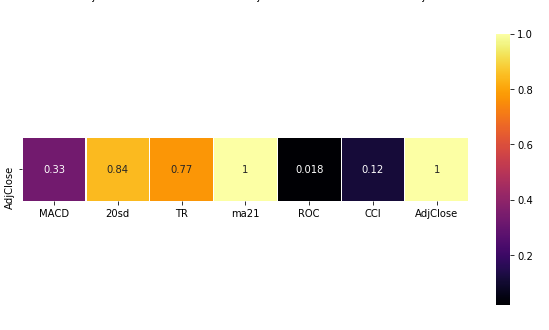
From the Heat Map we observe that the ma21 has perfect correlation with the AdjClose variable. Also 20sd and TR have positive correlation with the AdjClose, while the MACD and CCI don’t show significant correlation with AdjClose.

Lastly, we will use a method that is provided on the Random Forest algorithm  that gives information about the feature importance.  Firstly, we need to fit the model and then utilize the method called _feature_importance__ (these steps are explained in next sections, but here we want to inspect _feature_importance__ method ) on the model object.In the next line, we will fit a Random Forest Regressor model between the features and the target variable of the model, and extract the _features_importance__ method. Finally we make a bar plot of the features importance measure.

# Fit Random Forest Regressor and extract feature importance
prices = pd.DataFrame(amz['AdjClose'])
vars_model = prices.join(vars_)
vars_model= vars_model.dropna()
 
X = vars_model[['MACD','20sd','TR','ROC','CCI']].values
y = vars_model['AdjClose'].values
 
forest = RandomForestRegressor(n_estimators=1000)
forest = forest.fit(X, y)
importances = forest.feature_importances_
 
values = list(zip(vars_model.columns[1:],importances))
headers = ['feature','score']
values_df = pd.DataFrame(values,columns = headers)
 
# Plot the feature importance
columns = ['MACD','20sd','TR','ROC','CCI']
nd = np.arange(len(columns))
width=0.5
fig = plt.bar(nd, values_df['score'].values, color=sns.color_palette("deep", 5))
plt.legend(fig, columns, loc = 'upper right',bbox_to_anchor=(1.1, 1), title = "Feature Importance")
plt.show()

Figure 3: Feature Importance

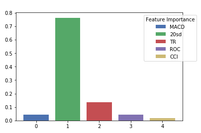
The bar plot of the feature importance show that 20sd has the greater importance in the prediction of the target variable AdjClose. On the second place comes the TR feature with significantly lower importance.

In this section we provided some tools to analyze the power prediction of the features before start to training a Machine Learning model. Is important to inspect the independent variables first for selecting the best features. 

After the inspection of the features, the next step consists in the training and testing steps where is necessary to split the data among  the train and test data. This is explained in the following section.