Decision Trees in Machine Learning

Decision tree is a popular Supervised learning algorithm which can handle classification and regression problems. For both problems, the algorithm breaks down a dataset into smaller subsets by using if-then-else decision rules within the features of the data. 

The general idea of a decision tree is that each of the features are evaluated by the algorithm and used to split the tree based on the capacity that they have to explain the target variable. The features could be categorical or continuous variables.  

In the process of building the tree, the most important features are selected by the algorithm in a top-down approach creating the decision nodes and branches of the tree and making predictions at points when the tree cannot be expanded any more. 

The tree is composed by a root node, decision nodes and leaf nodes. The root node is the top most decision on the tree, and is the first time where the tree is split based on the best predictor of the dataset. 

The decision nodes are the intermediate steps in the construction of the tree and are the nodes used to split the tree based on different values of the independent variables or features of the model. The leaf nodes represent the end points of the tree, and hold the prediction of the model.  

Decision Tree Structure

The methods to split the tree are different depending if we are in a classification or regression problem. We will provide an overview of the different measures that are used to split the tree in both types of problems.

Classification Problem

In this type of problem the algorithm decides which is the best feature to split the tree based on two measures that are Entropy and Information Gain. 

Entropy

Entropy is a coefficient that takes values between 0 and 1. It is a measure of randomness in data. If entropy is equal to zero, it means that all the data belongs to the same class, and if entropy is equal to 1, it means that half of the data belong to one class and the half belong to the other class (in binary classification). In this last situation, the data is perfect randomness.

The mathematical formula of entropy is as follows:

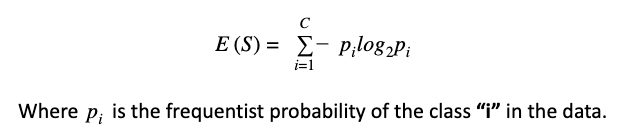
The goal of a decision tree problem is to reduce the measure of entropy while building the tree. As we stated above, entropy is a measure of the randomness of the data, and this measure needs to be reduced.  For this purpose, the entropy is combined with the Information Gain in order to select the feature that has higher value of Information Gain.

Information Gain

The Information gain is based on the decrease in E****ntropy after a dataset is split on an attribute or feature. The attribute that has the high value of Information Gain will be used to split the tree in nodes in a top-down approach.The mathematical formula of Information Gain is the following:

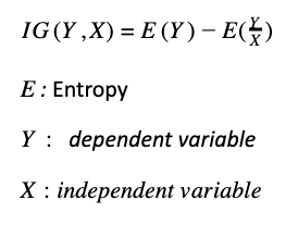
In the equation above, the Information Gain subtracts the entropy of the target variable Y given X (E(Y/X)) from the entropy of the target variable Y (EY), to calculate the reduction of uncertainty of Y given additional piece of information X.

The aim of the decision tree in this type of problem is to reduce the entropy of the target variable. For this, the decision tree algorithm would use the Entropy and the Information Gain of each feature to decide what attribute will provide more information (or reduce the uncertainty of the target variable). 

Decision Tree Regression Problem

In the regression problem, the tree is composed (like in the classification problem) with nodes, branches and leaf nodes, where each node represents a feature or attribute, each branch represents a decision rule and the leaf nodes represent an estimation of the target variable.

Contrary to the classification problem the estimation of the target variable in a regression problem is a continuous value and not a categorical value. The ID3 algorithm (Iterative Dichotomiser 3) can be used to construct a decision tree for regression which replace the Information Gain metric with the Standard Deviation Reduction (SDR). 

The Standard Deviation Reduction is based on the decrease in standard deviation after a dataset is split on an attribute. The tree will be split by the attribute with the higher Standard Deviation Reduction of the target variable.

The standard deviation is used as a measure of homogeneity of the data. The tree is built top-down from the root node and data is partitioned into subsets that contain homogeneous instances of the target variable. If the samples are homogeneous, its standard deviation is zero.

The mathematical formula of the Standard Deviation Reduction is the following:

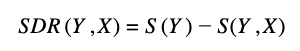
Y is target variable

X is a specific attribute of the dataset

SDRY,X is the reduction of the standard deviation of the target variable Y given the information of X

SY is the standard deviation of the target variable

S(Y,X)  is the standard deviation of the target variable given the information of X

The calculation of S(Y,X) can be broken down with the following formula that is important to understand the process:

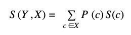
Sc is the standard deviation of the target variable based on unique values of the independent variable.

Pc  number of times (probability) of the value of the independent variables over the total values of the independent variable  

So the S(Y,X) is the sum of the probability of each of the values of the independent variable multiplied by the standard deviation of the target variable based on those values of the independent variable. 

The Standard deviation S(Y,X) is calculated for each feature or independent variable of the dataset. The feature with the great value of S(Y,X) is the feature that has more capability to explain the variations in the target variable, therefore is the feature that the decision tree algorithm will use to split the tree.

The same idea is that the feature that will be used to split the tree is the one that has the greatest Standard Deviation Reduction. The overall process of splitting a decision tree under the Standard Deviation Reduction can be synthetized in the following steps:

• Calculate the standard deviation of the target variable
• Calculate the Standard Deviation Reduction for all the independent variables
• The feature with the higher value on the Standard Deviation Reduction is chosen for the decision node.
• In each branch, the Coefficient Variation (CV) is calculated. This coefficient is a measure of homogeneity in the target variable. CV = Sx*100 (Standard deviation) /(mean of the target variable) * 100
•  If the CV is less than certain threshold such as 10% that subset does not need further splitting and the node become a leaf node.

Overfitting in Decision Tree

One of the most common problems with decision tree is that they tend to overfit a lot. There are situations where the tree is built with specific features of the training data and the predictive power for unseen data is reduced. 

This is because the branches of the tree follow strict and specific rules of the train dataset but for samples that are not part of the training set the accuracy of the model is not good. There are two main ways to address over-fitting in Decision tree. One is by using the Random Forest algorithm and the second is by pruning the tree.

Random Forest

Random Forest avoid overfitting as it is an ensemble of n decision trees (not just one) with n results in the end. The final result of Random forest is the most frequent response variable among the n results of the n Decision Trees if the target variable is a categorical variable or the average of the target variable in the leaf node if the target variable is a continuous variable.

Pruning

Pruning is done after the initial training is complete, and involves the removal of nodes and branches starting from the leaf nodes such that the overall accuracy is not affected.  The pruning technique will reduce the size of the tree by removing nodes that provide little power to classify or predict new instances.