Random Forest Model in R
Now, we will tune RandomForest model. Like SVM, we tune parameter based on 5% downsampling data. The procedure is exactly the same as for SVM model. Below we have reproduced the code for Random Forest model.
1set.seed(300)
2#down sampling again so than we get more info when stacking
3samp = downSample(data_train[-getIndexsOfColumns(data_train, c( "loan_status") )],data_train$loan_status,yname="loan_status")
4#choose small data for tuning
5train_index_tuning = createDataPartition(samp$loan_status,p = 0.05,list=FALSE,times=1)
6#choose small data for re-train
7train_index_training = createDataPartition(samp$loan_status,p = 0.1,list=FALSE,times=1)
8rfGrid = expand.grid(
9                .mtry = as.integer(seq(2,ncol(samp), (ncol(samp) - 2)/4))
10                )
11#Install random forest package
12library(randomForest)
13rfTuned = train(
14    samp[train_index_tuning,-getIndexsOfColumns(samp,"loan_status")],
15    y = samp[train_index_tuning,"loan_status"],
16    method = "rf",
17    tuneGrid = rfGrid,
18    metric = "ROC",
19    trControl = ctrl,
20    preProcess = NULL,
21    ntree = 100
22    )
23plot(rfTuned)
24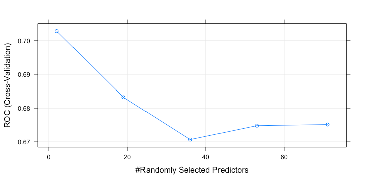
1> rfTuned
2Random Forest
31268 samples
4  70 predictor
5   2 classes: 'Default', 'Fully.Paid'
6No pre-processing
7Resampling: Cross-Validated (3 fold)
8Summary of sample sizes: 845, 845, 846
9Resampling results across tuning parameters:
10  mtry  ROC        Sens       Spec
11   2    0.7028532  0.6909073  0.6199440
12  19    0.6832394  0.6451832  0.6088706
13  36    0.6706683  0.6231333  0.5820516
14  53    0.6748038  0.6263003  0.6026111
15  71    0.6751421  0.6609511  0.5962622
16ROC was used to select the optimal model using the largest value.
17The final value used for the model was mtry = 2.
18>
19
The best parameter is mtry(number of predictors) = 2. Like SVM, we fit 10% of downsampling data with this value.
1rf_model = randomForest(loan_status ~ . ,data = samp[train_index_training,],mtry = 2,ntree=400)
2predict_loan_status_rf = predict(rf_model,data_test,"prob")
3predict_loan_status_rf = as.data.frame(predict_loan_status_rf)$Fully.Paid
4rocCurve_rf = roc(response = data_test$loan_status,
5               predictor = predict_loan_status_rf)
6auc_curve = auc(rocCurve_rf)
7plot(rocCurve_rf,legacy.axes = TRUE,print.auc = TRUE,col="red",main="ROC(RandomForest)")
8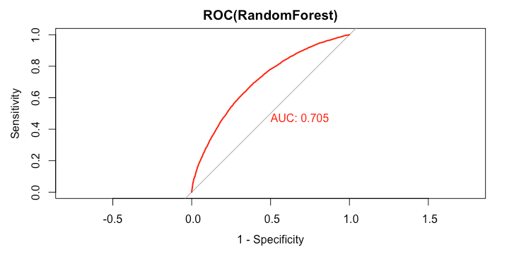
1> rocCurve_rf
2
3Call:
4roc.default(response = data_test$loan_status, predictor = predict_loan_status_rf)
5
6Data: predict_loan_status_rf in 5358 controls (data_test$loan_status Default) < 12602 cases (data_test$loan_status Fully.Paid).
7Area under the curve: 0.705
8>
9predict_loan_status_label = ifelse(predict_loan_status_rf<0.5,"Default","Fully.Paid")
10c = confusionMatrix(predict_loan_status_label,data_test$loan_status,positive="Fully.Paid")
11
12table_perf[3,] = c("RandomForest",
13  round(auc_curve,3),
14  as.numeric(round(c$overall["Accuracy"],3)),
15  as.numeric(round(c$byClass["Sensitivity"],3)),
16  as.numeric(round(c$byClass["Specificity"],3)),
17  as.numeric(round(c$overall["Kappa"],3))
18  )
19
The model’s performance is as follow:
1> tail(table_perf,1)
2         model   auc accuracy sensitivity specificity kappa
33 RandomForest 0.705    0.657       0.666       0.635 0.268
4>
5