A support vector machine (SVM) is a supervised learning technique that analyzes data and isolates patterns applicable to both classification and regression. The classifier is useful for choosing between two or more possible outcomes that depend on continuous or categorical predictor variables. Based on training and sample classification data, the SVM algorithm assigns the target data into any one of the given categories. The data is represented as points in space and categories are mapped in both linear and non-linear ways.

For SVM, we use Radial Basis as a kernel function. Due to limited computation reason, we use 5% of downsampling data for tuning parameter and 10% of downsampling data for training.

set.seed(200)
samp = downSample(data_train[-getIndexsOfColumns(data_train, c( "loan_status") )],data_train$loan_status,yname="loan_status")
> table(samp$loan_status)

   Default Fully.Paid 
     12678      12678 
> 

#choose small data for tuning 
train_index_tuning = createDataPartition(samp$loan_status,p = 0.05,list=FALSE,times=1)
#choose small data for re-train
train_index_training = createDataPartition(samp$loan_status,p = 0.1,list=FALSE,times=1)

library(“kernlab”)
svmGrid = expand.grid(
                .sigma = as.numeric(sigest(loan_status ~.,data = samp[train_index_tuning,],scaled=FALSE)),
                .C = c(0.1,1,10)
                )

svmTuned = train(
    samp[train_index_tuning,-getIndexsOfColumns(samp,"loan_status")],
    y = samp[train_index_tuning,"loan_status"],
    method = "svmRadial",
    tuneGrid = svmGrid,
    metric = "ROC",
    trControl = ctrl,
    preProcess = NULL,
    scaled = FALSE,
    fit = FALSE)

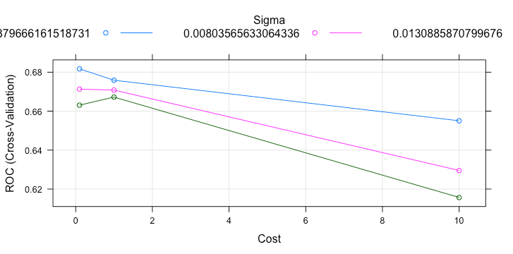
plot(svmTuned)

> svmTuned
Support Vector Machines with Radial Basis Function Kernel 
1268 samples
  70 predictor
   2 classes: 'Default', 'Fully.Paid' 
No pre-processing
Resampling: Cross-Validated (3 fold) 
Summary of sample sizes: 845, 845, 846 
Resampling results across tuning parameters:
  sigma        C     ROC        Sens       Spec     
  0.003796662   0.1  0.6817007  0.5912024  0.6639021
  0.003796662   1.0  0.6758736  0.6261886  0.6388193
  0.003796662  10.0  0.6550318  0.6151599  0.5899431
  0.008035656   0.1  0.6713062  0.5851292  0.6751244
  0.008035656   1.0  0.6708204  0.6277907  0.6072610
  0.008035656  10.0  0.6295020  0.5946899  0.5789442
  0.013088587   0.1  0.6630773  0.6025217  0.6261960
  0.013088587   1.0  0.6672180  0.6356523  0.5978122
  0.013088587  10.0  0.6156558  0.6041164  0.5615667
ROC was used to select the optimal model using the largest value.
The final values used for the model were sigma = 0.003796662 and C = 0.1.
>

The best parameter for the model is sigma = 0.003796662, and C = 0.1. We use this values to fit the 10% of downsampling data and collect its performance based on test set.

svm_model = ksvm(loan_status ~ .,
                 data = samp[train_index_training,],
                 kernel = "rbfdot",
                 kpar = list(sigma=0.003796662),
                 C = 0.1,
                 prob.model = TRUE,
                 scaled = FALSE)

Prediction

predict_loan_status_svm = predict(svm_model,data_test,type="probabilities")
predict_loan_status_svm = as.data.frame(predict_loan_status_svm)$Fully.Paid

ROC and AUC

rocCurve_svm = roc(response = data_test$loan_status,
               predictor = predict_loan_status_svm)
auc_curve = auc(rocCurve_svm)
> plot(rocCurve_svm,legacy.axes = TRUE,print.auc = TRUE,col="red",main="ROC(SVM)")

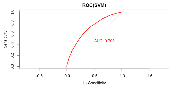
> auc_curve
Area under the curve: 0.7032

predict_loan_status_label = ifelse(predict_loan_status_svm<0.5,"Default","Fully.Paid")
c = confusionMatrix(predict_loan_status_label,data_test$loan_status,positive="Fully.Paid")

This is the summary of model’s performance.

table_perf[2,] = c("SVM",
  round(auc_curve,3),
  as.numeric(round(c$overall["Accuracy"],3)),
  as.numeric(round(c$byClass["Sensitivity"],3)),
  as.numeric(round(c$byClass["Specificity"],3)),
  as.numeric(round(c$overall["Kappa"],3))
  )

> tail(table_perf,1)
  model   auc accuracy sensitivity specificity kappa
2   SVM 0.703    0.635       0.612       0.688 0.257
>