To build our first model, we will tune Logistic Regression to our training dataset.

First we set the seed (to any number. we have chosen 100) so that we can reproduce our results.

Then we create a downsampled dataset called samp which contains an equal number of Default and Fully Paid loans. We can use the table() function to check that the downsampling is done correctly.

> set.seed(100)
> samp = downSample(data_train[-getIndexsOfColumns(data_train, c( "loan_status") )],data_train$loan_status,yname="loan_status")
> table(samp$loan_status)
   Default Fully.Paid 
     12678      12678 
>

We will now choose a small set of data for tuning the model.

#choose small data for tuning
train_index = createDataPartition(samp$loan_status,p = 0.05,list=FALSE,times=1)

We will use the functions available in the caret package to train the model.

Step 1: We setup the control parameter to train with the 3-fold cross validation (cv)

ctrl <- trainControl(method = "cv",
    summaryFunction = twoClassSummary,
    classProbs = TRUE,
    number = 3
    )

Step 2: We train the classification model on the data

glmnGrid = expand.grid(.alpha = seq(0, 1, length = 10), .lambda = 0.01)
glmnTuned = train(samp[train_index,-getIndexsOfColumns(samp,"loan_status")],y = samp[train_index,"loan_status"],method = "glmnet",tuneGrid = glmnGrid,metric = "ROC",trControl = ctrl)

Advanced Notes

We use Elastic Net regularization, which comprises of Ridge and Lasso regularization, with cross-validation to prevent overfitting. Our goal is maximizing AUC. Learn more about Regularization here.

Due to limited computation resource, we run model tuning on small data and fixed lambda parameter. We use small fold: 3-fold cross validation. We then refit the best model with the whole data.

(Note: we put the final tuning result here instead of running through the whole process. We disable the execution of tuning code although readers can enable it back by setting eval = TRUE )

Look Inside glmTuned

We can now examine the output of the generated model.

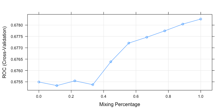
plot(glmnTuned)

> glmnTuned
glmnet 
1268 samples
  70 predictor
   2 classes: 'Default', 'Fully.Paid' 
No pre-processing
Resampling: Cross-Validated (3 fold) 
Summary of sample sizes: 846, 844, 846 
Resampling results across tuning parameters:
  alpha      ROC        Sens       Spec     
  0.0000000  0.6754917  0.6261588  0.6261215
  0.1111111  0.6753332  0.6245939  0.6261215
  0.2222222  0.6755427  0.6293332  0.6340055
  0.3333333  0.6753729  0.6277609  0.6371725
  0.4444444  0.6763833  0.6277609  0.6356002
  0.5555556  0.6772067  0.6277609  0.6387523
  0.6666667  0.6774650  0.6230290  0.6387746
  0.7777778  0.6777457  0.6214567  0.6372023
  0.8888889  0.6780438  0.6230365  0.6372023
  1.0000000  0.6782664  0.6277758  0.6356300
Tuning parameter 'lambda' was held constant at a value of 0.01
ROC was used to select the optimal model using the largest value.
The final values used for the model were alpha = 1 and lambda = 0.01.
>

The best penalty parameter is alpha = 1 (more weight on Ridge) with fixed shrinking lambda = 0.01. We use this parameter to retrain the whole sample.

library(glmnet)
model = glmnet(
    x = as.matrix(samp[-getIndexsOfColumns(samp,"loan_status")]),
    y=samp$loan_status,
    alpha = 1,
    lambda = 0.01,
    family = "binomial",
    standardize = FALSE)

The finalized Logistic Regression model is applied to the test loan data. We look at ROC graph and AUC. We also set probability prediction cutoff at 50% (noted that the higher this value is, the more likely the loan is Fully Paid) and collect some performance metrics for a later comparison.

table_perf = data.frame(model=character(0),
                        auc=numeric(0),
                        accuracy=numeric(0),
                        sensitivity=numeric(0),
                        specificity=numeric(0),
                        kappa=numeric(0),
                        stringsAsFactors = FALSE
                        )

predict_loan_status_logit = predict(model,newx = as.matrix(data_test[-getIndexsOfColumns(data_test,"loan_status")]),type="response")

ROC and AUC

library(pROC)
rocCurve_logit = roc(response = data_test$loan_status,
               predictor = predict_loan_status_logit)
auc_curve = auc(rocCurve_logit)

plot(rocCurve_logit,legacy.axes = TRUE,print.auc = TRUE,col="red",main="ROC(Logistic Regression)"

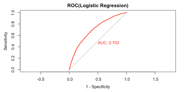
> rocCurve_logit
Call:
roc.default(response = data_test$loan_status, predictor = predict_loan_status_logit)
Data: predict_loan_status_logit in 5358 controls (data_test$loan_status Default) < 12602 cases (data_test$loan_status Fully.Paid).
Area under the curve: 0.7031
>

> predict_loan_status_label = ifelse(predict_loan_status_logit<0.5,"Default","Fully.Paid")
> c = confusionMatrix(predict_loan_status_label,data_test$loan_status,positive="Fully.Paid")
> table_perf[1,] = c("logistic regression",
  round(auc_curve,3),
  as.numeric(round(c$overall["Accuracy"],3)),
  as.numeric(round(c$byClass["Sensitivity"],3)),
  as.numeric(round(c$byClass["Specificity"],3)),
  as.numeric(round(c$overall["Kappa"],3))
  )
> rm(samp,train_index)
> tail(table_perf,1)
                model   auc accuracy sensitivity specificity kappa
1 logistic regression 0.703    0.645       0.643        0.65 0.256
>