A matrix is a table of numbers. In math text, it is conventional to denote matrices with bold letters. For example, consider a matrix D of the prices of the securities on first three days of the week.
1D =2643136528466355
Test Your Knowledge
Check your understanding of this lesson with a short quiz.
This matrix is {3\*2} matrix (pronounced "3 by 2") . The number of rows is given first, followed by the number of columns. The Matrix D shows that on the first day, the bond was worth $64 and the stock was worth $31. On the second day the bond was worth $65 and the stock $28. On the third day the bond was worth $66 and the stock $35.
With this data in place, we can answer many analytics questions considering someone was holding these assets in their portfolio. Let's learn how to use matrices in R and then how to perform statistical analysis on them.
Defining a Matrix in R
Let's say we have the above data in the form of a vector:
> price_data <- c(64,31,65,28,66,35)
We know that this data represents three rows with each row containing the bond price and the stock price. In R, we can use this vector to create a matrix using the matrix() function as shown below:
1#price data each number pair represents the bond an dstock price2price_data <- c(64,31,65,28,66,35)3#Create matrix of prices4price_matrix <- matrix(price_data, nrow=3,byrow=TRUE)5#print the matrix6price_matrix
7
Matrix function parameters:
The first argument is the data that the matrix function will convert into rows and columns.
The second argument nrow indicates that the matrix will have three rows. A similar argument ncol could be used to indicate the number of columns.
The third argument byrow indicates how the data should be processed. byrow=TRUE indicates that it should be processed by row, i.e., as data comes in it will first fill the first row, then second and so on. To process data by columns, byrow should be set to FALSE.
When this matrix is printed, it will look as follows:
Currently our matrix doesn't have any names for the rows and columns and it's difficult to understand the data. Our first column represents the prices of the bond and the second column represents the prices of stock. The three rows represent three days, namely, Mon, Tue and Wed.
In R, we can assign names to the matrix using the rownames() and colnames() functions as shown below:
1#set row names and column names for price_matrix2rownames(price_matrix)<- c("Mon","Tue","Wed")3colnames(price_matrix)<- c("Bond","Stock")4#print the matrix5price_matrix
6
We can now print the matrix:
1> price_matrix
2 Bond Stock
3Mon 64314Tue 65285Wed 66356>7
Another easy way to assign names to a matrix is to use the dimnames() function, as shown below. Note the use of list() function which we will discuss in the upcoming lessons. This list has two objects, the first is the vector for row names and the second is the vector for column names.
1#Use the dimnames function to assign names to matrix elements2dimnames(price_matrix)<-list(c("Mon","Tue","Wed"),c("Bond","Stock"))3#print the matrix4price_matrix
5
Selecting the Matrix Elements
We can select specific elements of a matrix by using the expression D[m, n], i.e., mth row and nth column of matrix D.
Below R script shows some different ways of selecting the matrix elements:
1>#print the matrix2> price_matrix
3 Bond Stock
4Mon 64315Tue 65286Wed 66357>8>#What is the bond price on 3rd day? (3rd row and 1st column)9> price_matrix[3,1]10[1]6611>12>#Get me just the stock prices for all days13>#In this case we want to access all rows, so we will just omit supplying the row14>#stock prices are in 2nd column15> price_matrix[,2]16Mon Tue Wed
1731283518>19>#Get stock and bond price on Tuesday20>#Tuesday is the 2nd row21> price_matrix[2,]22 Bond Stock
23652824>25>#Get all prices for Monday and Wednesday26>#Monday and Wednesday data is in row 1 and 327> price_matrix[c(1,3),]28 Bond Stock
29Mon 643130Wed 663531>32>#Get stock prices for Tuesday and Wednesday33>#We can use colon for continuing elements34> price_matrix[2:3,2]35Tue Wed
36283537>38
Arithmetic Operations on Matrices
Just like vectors, we can use standard operators +, -, /, * with matrices. Let's take a few examples to understand the matrix arithmetic and also understand a few other matrix operations along the way.
Let's say that you hold 5 quantity each of this bond and stock. We can multiple the price_matrix to get the dollar holding value of your assets. We store this in the matrix portfolio_value.
Now that we have the portfolio values, we can calculate the total portfolio value on each day by adding the value of stocks and bonds. This can be done using the rowSums() function. We store the results in a vector called days_total.
We now have a new vector which contains daily portfolio value totals. But it is not a part of the portfolio_value matrix. We can add the days_total vector to the main matrix using cbind() function.
Since we have the portfolio values over a three day period, we can calculate the average portfolio value during this period. The values are in columns so we can use colMeans() function to calculate the column means. We store these values in a vector called days_average.
Finaly we can add the days_average vector as a new row to our main matrix. Since we are adding a row, we will use rbind() function.
The resulting matrix contains portfolio values along with totals and average over a period of three days.
1>#print the matrix2> price_matrix
3 Bond Stock
4Mon 64315Tue 65286Wed 66357>8>#You hold 5 quantity ech of bond and stock. What is the value?9> portfolio_value <- price_matrix *510>11>#What is the total portfolio value on each day12> days_total <- rowSums(portfolio_value)13>14>#print days total15> days_total
16Mon Tue Wed
1747546550518>19>#We can added the days_total vector to the main matrix using cbind()20> portfolio_value_totals <- cbind(portfolio_value,days_total)21>22>#Calculate average value per day23> days_average <- colMeans(portfolio_value_totals)24>25>#Add the averages row to the portfolio_value_totals matrix26> final_matrix <-rbind(portfolio_value_totals,days_average)27>28>#print final_matrix29> final_matrix
30 Bond Stock days_total
31Mon 320155.0000475.000032Tue 325140.0000465.000033Wed 330175.0000505.000034days_average 325156.6667481.666735>36
Multiplying Matrix with a Vector
In the above example, we assumed the same quantity 5 for both stock and bond and simply multiplied it with the matrix. R took care of multiplying each matrix element with 5 to get us the values. However, what if we have different quantities of stock and bond. In such a case we can store the quantities in a new vector and then do standard matrix multiplication to achieve our results. Note that what we did earlier (multiply by *) is not the standard matrix multiplication for which you should use %*% in R. The calculation and nuances are demonstrated below:
1#print the matrix2price_matrix
3# Assign quantities - 5 bonds and 3 stocks4quantities <-c(5,3)5# Multiply prices with quantities to get the values.6portfolio_value <- price_matrix %*% diag(quantities)7
%*% represents standard matrix multiplication.
diag() create a diagnal matrix from the vector so that we can then multiply the two matrices.
Multiplying the price matrix with the quantity vector will look as follows:
Note: If you did not understand this calculation, don't worry about it at this stage. We will learn a lot more about matrix multiplication in future courses. The objective of bringing this up here was to just familiarize you with the possibilities of the advance calculations that can be done.
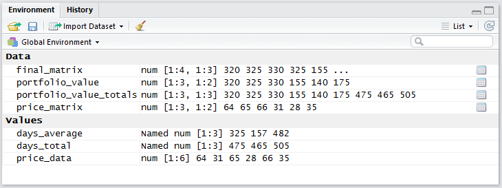
When you create a new vector, matrix or any other R object, it gets saved into the workspace and is available for you to use in your calculations. These variables can be seen in the Global Environment, i.e., the top-right window in RStudio. You can also access all objects available in the workspace using the ls() command in R console.