Simulate White Noise (WN) in R

The function arima.sim() can be used to simulate data from a variety of time series models. Based on the model we want to apply, we specify the appropriate values for p, d and q to the model ARIMA(p,d,q).

The general format for the arima.sim() function is as follows:

arima.sim(model, n)
model is where we specify the AR, differencing order and MA components.
n is the length of output series.

For the White Noise model, all p, d and q in arima model are 0. So, ARIMA(0,0,0) is simply the White Noise(WN) model.

Simulate White Noise Model in R

To simulate WN model in R, we will set all, p, d and q to 0. To generate 200 observation series, we will set the n argument to 200.

WN <- arima.sim(model = list(order = c(0, 0, 0)), n = 200)

This will create a time series object that follows White Noise model.

You can plot the newly generated time series using the plot.ts() function.

> plot.ts(WN,col=4, main="White Noise Series")

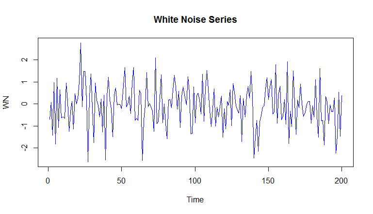
You can calculate the mean and standard deviation of this series and notice that the series will have a mean close to 0 and a standard deviation close to 1.

> mean(WN)
[1] -0.08357315
> var(WN)
[1] 0.91063
> sd(WN)
[1] 0.9542694

While generating the White Noise series, we can also specify the mean and standard deviation. In the following example, we simulate White Noise model with mean=50 and sd=10.

> WN_2 <- arima.sim(model = list(order = c(0, 0, 0)), n = 200, mean=50, sd=10)
> plot.ts(WN_2,col=4, main="White Noise Series (mean=50, sd=10)")

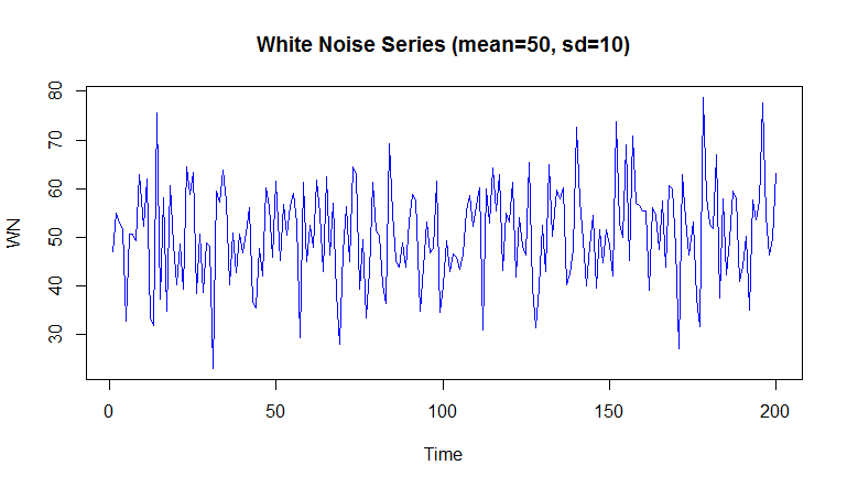
Again, we can verify that the statistics for this time series are close to what we fed to it.

> mean(WN_2)
[1] 50.64454
> sd(WN_2)
[1] 10.0867
>

Estimating the White Noise Model (Model Fitting)

If we have a series (where we feel White Noise model is suitable), then we can fit the White Noise model using the arima() function. When applied, the arima() function returns the important information about the estimated model, such as its estimated mean and variance.

We will use the White Noise series, WN, that we created above to fit the model to it.

> arima(WN, order = c(0, 0, 0))
Call:
arima(x = WN, order = c(0, 0, 0))
Coefficients:
      intercept
        50.6445
s.e.     0.7115
sigma^2 estimated as 101.2:  log likelihood = -745.53,  aic = 1495.06
>

The intercept 50.6445 is the mean and sigma^2 101.2 is the variance, which gives a standard deviation, sigma of 10.05982. Compare this with the mean and standard deviation we calculated using the standard mean() and sd() functions.