Simulate Random Walk (RW) in R

When a series follows a random walk model, it is said to be non-stationary. We can stationarize it by taking a first-order difference of the time series, which will produce a stationary series, that is, a Zero Mean White Noise series. For example, the stock prices of a stock follow a random walk model, and the series of returns (differencing of pricing series) will follow White Noise model.

Let's understand this phenomenon in more detail.

Since the differencing of a Random Walk series is a White Noise series, we can say that a Random Walk series is a cumulative sum (i.e., Integration) of a zero mean White Noise series. With this information, we can define Random Walk series in the form of ARIMA model as follows:

1ARIMA(0,1,0)
2Where:
3- Augoregressive part, p = 0
4- Integration, d = 1
5- Moving average part, q = 0
6

Simulate Random Walk Series

We can now simulate a random walk series in R by supplying the appropriate parameters to the arima.sim() function as shown below:

1RW <- arima.sim(model= list(order = c(0, 1, 0)), n=200)
2

We can plot the newly generated series using the plot.ts() function.

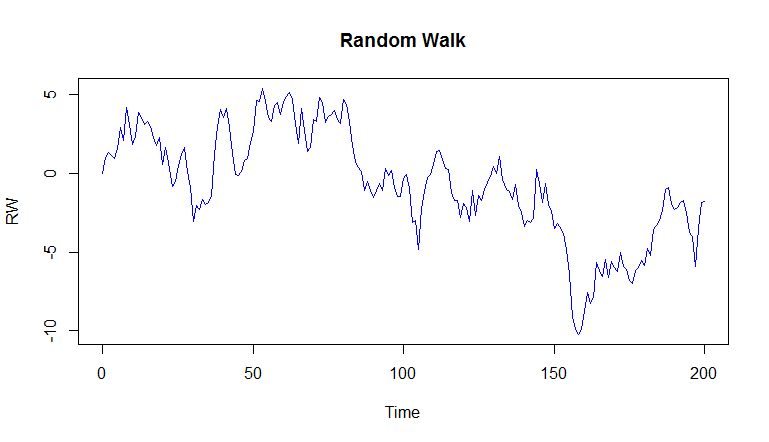
As we can clearly observe, this is a non-stationary series and its mean and standard deviation is not constant over time.

First Difference Series

In order to make the series stationary, we take the first order difference of the series.

When plotted you will notice that the difference series resembles White Noise.

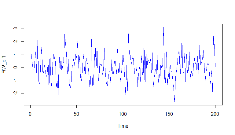
The statistics for the RW_diff series are calculated below:

1> mean(RW_diff)
2[1] -0.00903282
3> sd(RW_diff)
4[1] 1.020447
5>
6

Random Walk with Drift

The above Random Walk series that we simulated wanders up and down around the mean. However, we can have the Random Walk series follow an up or a down trend, called drift. To do so, we provide an additional argument mean/intercept to the arima.sim() function. This intercept is the slope for the model. We can also change the standard deviation of the simulated series. In the following code, we supply a mean of 1 and a standard deviation of 5.

1> RW_drift <- arima.sim(model= list(order = c(0, 1, 0)), n=200, mean=1,sd=5)
2> plot.ts(RW_drift, main="Random Walk with Drift")
3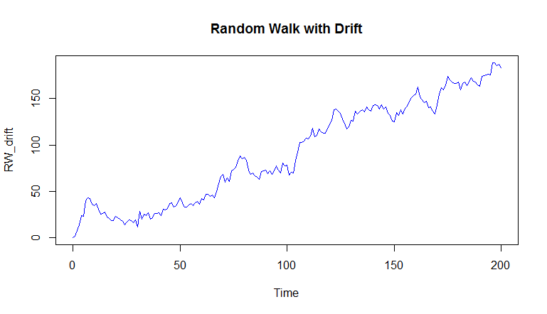

Estimating Random Walk Model

To fit a random walk model with a drift to a time series, we will follow the following steps

1. Take the first order difference of the data.
2. Fit the white noise model to the differenced data using arima() function with order of c(0,0,0).
3. Plot the original time series plot.
4. Add the estimated trend using the abline() function by supplying the intercept we got by fitting the White Noise model as the slope.

1. First Order Difference

In order to make this series stationary, we will take the difference of the series.

1> RW_drift_diff <-diff(RW_drift)
2> plot.ts(RW_drift_diff, col=4, main="First Order Difference")
3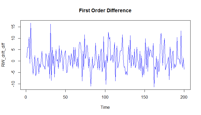

2. Fit White Noise model to differenced data

We can now use the arima() function to fit the White Noise model to the differenced data.

1> whitenoise_model <- arima(RW_drift_diff, order = c(0, 0, 0))
2> whitenoise_model
3Call:
4arima(x = RW_drift_diff, order = c(0, 0, 0))
5Coefficients:
6      intercept
7         0.9189
8s.e.     0.3631
9sigma^2 estimated as 26.37:  log likelihood = -611.01,  aic = 1226.01
10>
11

We can see that the fitted White Noise model has an intercept of 0.9189.

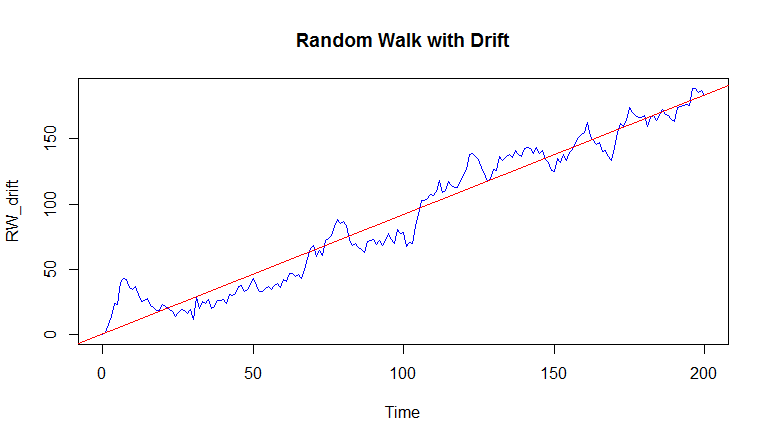
3. Plot the original Random Walk data

This can be done using the following command:

1> plot.ts(RW_drift,col=4, main="Random Walk with Drift")
2

4. Add the estimated trend

Now on the same plot we want to add the estimated trend. At the beginning of this lesson we explained how a Random Walk series is a cumulative sum (i.e., Integration) of a zero mean White Noise series. So, the intercept, in effect, is actually the slope for our random walk series.

We can plot the trend line using the abline(a,b) function, where a is the intercept and b is the slope of the line. In our case, we will specify 'a=0' and 'b=intercept' of the White Noise model.

The estimated trend line will be added to our plot.