Now that we know how to estimate the AR model using ARIMA, we can create a simple forecast based on the model.

Step 1: Fit the model

The first step is to fit the model as ARIMA(1, 0, 0). We have already seen this in the previous lesson.

> msft_ar<-arima(msft_ts,c(1,0,0))

Step 2: Create Forecast

We can now use the predict() function to create a forecast using the fitted AR model. It takes as its inputs, the model object that we created in step 1, and an additional parameter n.ahead which establishes the forecast horizon, that is, how many steps (periods) in the future we want to create the forecast. In our example, we will provide n.ahead=20, which will create forecast for next 20 steps which corresponds to 20 days for our daily data.

> msft_forecast <- predict(msft_ar, n.ahead = 20)

The object generated by the predict() command contains two time series: 1) $pred which contains the forecasted values and 2) $se which contains the standard error for the forecast. We will use the $pred time series to plot the forecast and the $se time series to add confidence intervals to our plot.

> msft_forecast pred Time Series: Start = 253 End = 272 Frequency = 1 \[1\] 62.03064 61.92331 61.81796 61.71456 61.61307 61.51346 61.41569 \[8\] 61.31973 61.22554 61.13309 61.04236 60.95330 60.86588 60.78009 \[15\] 60.69588 60.61323 60.53210 60.45248 60.37432 60.29762 se Time Series: Start = 253 End = 272 Frequency = 1 [1] 0.7675185 1.0754465 1.3051026 1.4933081 1.6544932 1.7961449 [7] 1.9227626 2.0373125 2.1418796 2.2379995 2.3268456 2.4093400 [13] 2.4862246 2.5581077 2.6254964 2.6888192 2.7484426 2.8046829 [19] 2.8578161 2.9080845

For simplicity sake, let's also extract the two series in their own respective variables.

> msft_forecast_values <- msft_forecast$pred

msft_forecast_se <- msft_forecast$se

Step 3: Plot the Forecast

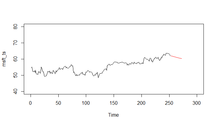
We can now use the plot.ts() function to first plot the original data and then add points for the forecasted values using the points() function as shown below:

> plot.ts(msft_ts, xlim = c(0, 300), ylim = c(40,80))

points(msft_forecast_values , type = "l", col = 2)

Notice that while creating the initial plot, we've specified scale limits for x and y axis in order to provision for the forecast values.

Step 4: Add Confidence Intervals to Forecast

We can add a 95% confidence interval to our forecast using the standard error values.

> points(msft_forecast_values - 2*msft_forecast_se, type = "l", col = 4, lty = 2)

points(msft_forecast_values + 2*msft_forecast_se, type = "l", col = 4, lty = 2)

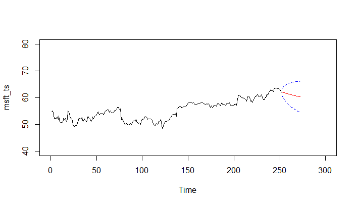
You have successfully created your first forecast.