We will now see how we can fit an MA model to a given time series using the arima() function in R. Recall that MA model is an ARIMA(0, 0, 1) model.

We can use the arima() function in R to fit the MA model by specifying order = c(0, 0, 1).

We will perform the estimation using the msft_ts time series that we created earlier in the first lesson. If you don't have the msft_ts loaded in your R session, please follow the steps to create it as specified in the first lesson.

Let's start by creating a plot of the original data using the plot.ts() function.

> plot.ts(msft_ts, main="MSFT prices", ylab="Prices")

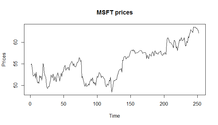
We will fit the MA model to this data using the following command:

msft_ma <- arima(msft_ts, order = c(0, 0, 1))

The output contains many things including the estimated slope (ma1), mean (intercept), and innovation variance (sigma^2) as shown below:

> msft_ma
Call:
arima(x = msft_ts, order = c(0, 0, 1))
Coefficients:
         ma1  intercept
      0.8602    55.2735
s.e.  0.0259     0.2603
sigma^2 estimated as 4.952:  log likelihood = -559.83,  aic = 1125.66
>

The msft_ma object also contains the residuals (εt ). We can extract the residuals, using the residuals() function in R.

residuals <- residuals(msft\_ma)

Once you find the residuals εt, the fitted values are just X̂_t=X_t−ε_t. In R, we can do it as follows:

msft_fitted <- msft_ts - residuals

We can now plot both the original and the fitted time series to see how close the fit is.

ts.plot(msft_ts)
points(msft_fitted, type = "l", col = 2, lty = 2)

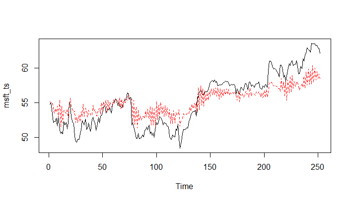
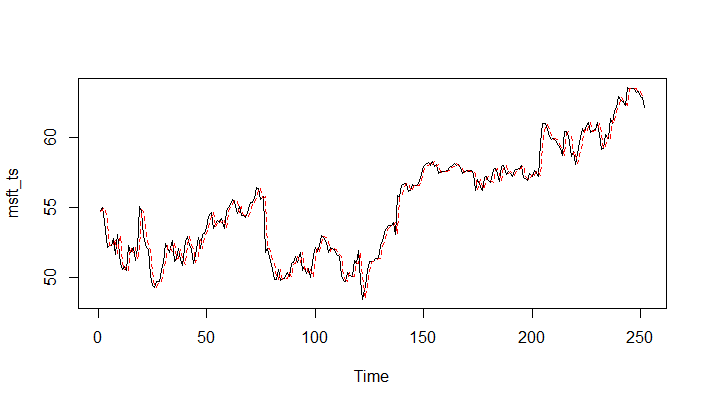
As we can see, the model does not provide a good fit for the original series. One possible reason is that our original series was not stationary. We can fit the ARIMA model with first order differencing by passing the parameter I=1.

> msft_ma <- arima(msft_ts, order = c(0, 1, 1))
> residuals <- residuals(msft_ma)
> msft_fitted <- msft_ts - residuals
> ts.plot(msft_ts)
> points(msft_fitted, type = "l", col = 2, lty = 2)