Constructing an Efficient Frontier

This lesson is part 2 of 8 in the course Understanding Portfolio Math

The concept of Efficient Frontier was first introduced by Harry Markowitz in his paper on Portfolio Selection (1952 Journal of Finance).

The portfolio theory considers a universe of risky investments and explores these possible investments in order to find the optimum portfolio. So, for a given amount of risk, MTP explains how select a portfolio with maximum returns, and with a given amount of return, MTP explains how to select a portfolio with minimum risk.

Suppose you have all the required data (expected returns, volatility, and correlations) for all the investments you are considering. Using this data, you can create various portfolios with different portfolio risk and return profiles.

Among all these portfolios, choose the optimal portfolios in either of the following way:

Identify all the portfolios that have the same risk (volatility). From this sub-set of portfolios, choose the one that has the highest return.
Identify all the portfolios that have the same returns. From this sub-set of portfolios, choose the one that has the lowest risk.

Both the methods will product a set of optimal portfolios. This set of optimal portfolios is called the efficient frontier. (Later in this post, we will learn how to construct an efficient frontier in Excel)

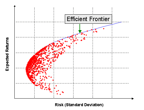
If you plot all the portfolios that you could make using the universe of risky securities that you have, the graph will look something like the one below:

Each red dot represents the mean and standard deviation of a portfolio. The blue line is the efficient frontier. The efficient frontier has all the optimal portfolios we selected above. Portfolios on the efficient frontier have maximum return for a given level of risk or, alternatively, minimum risk for a given level of return. Clearly, a rational investor will select a portfolio on the efficient frontier.

Dominated Portfolio

In the above graph, you see that for the same level of risk there are multiple portfolios providing different levels of return. A portfolio is said to be dominated, if there is atleast one portfolio that has higher return and lower standard deviation. In other words, a portfolio is dominated if there is any other portfolio to its north-west. So, in the above graph, all portfolios other than those on the efficient frontier are dominated.

Typically, the portfolios that make the efficient frontier are the most diversified ones. Less diversified portfolios tend to be closer to the middle of the achievable region.