AutoRegressive (AR) model is one of the most popular time series model. In this model, each value is regressed to its previous observations. AR(1) is the first order autoregression meaning that the current value is based on the immediately preceding value.

We can use the arima.sim() function to simulate the AutoRegressive (AR) model.

Note that model argument is meant to be a list giving the ARMA order, not an actual arima model. So, for the AutoRegressive model, we will specify model as list(ar = phi) , in which phi is a slope parameter from the interval (-1, 1).

Below we create two sets of simulations with AR model, one with a slope of 0.5 and another with a slope of 0.8.

# Simulate AutoRegressive model with 0.5 slope
AR_1 <- arima.sim(model = list(ar = 0.5), n = 200)
# Simulate AutoRegressive model with 0.8 slope
#
AR_2 <- arima.sim(model = list(ar = 0.9), n = 200)
plot.ts(cbind(AR_1 , AR_2 ), main="AR Model Simulated Data")

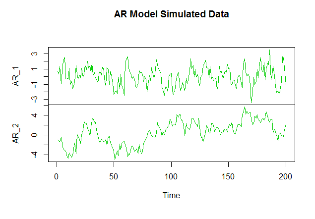
It is important to note that Random Walk is a special case of AutoRegressive models, where the slope parameter is equal to 1.

ACF and PACF of Autoregressive Model

We can calculate the Autocorrelation and Partial Autocorrelation Functions of the Autoregressive model using the acf() and the pacf() functions.

The following are the respective ACF and PACF plots for the AR_1 series.

> acf(AR_1)
> pacf(AR_1)

Characteristics of AutoRegressive Model

Persistence: The slope in an AR model can range from -1 to 1. As the slope gets closer to 1, the model shows higher persistence, i.e., it shows higher correlation with previous values. Also, the higher the slope, the slower is the decay of ACF to 0.

Oscillatory behavior: This refers to a large amount of variation between an observation and its lag. As the slope reduces, the AR model exhibits oscillatory behavior.