Aggregating Demand and Supply Curves and Concept of Equilibrium

Qd = 415*1000 – 1.2P*1000 = 415,000 – 1,200P

The inverse demand function will be:

P = 415,000/1,200 - Qd/1200, or

P = 345.83 – 0.0008 Qd

-0.0008 is the slope of the aggregate demand curve.

Similarly if the supply function for a product is Qs = 400+1.5P and there are 100 manufacturers of the product, the market supply will be:

Qs = 40,000+150P

The inverse market supply function will be:

P = - 266.67 + 0.0067Qs

0.0067 is the slope of the aggregate supply curve.

Market Equilibrium

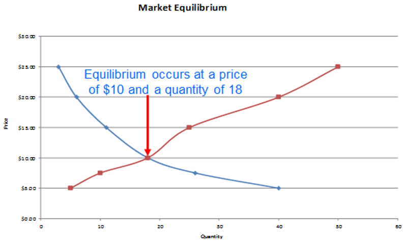
Using the market supply and the market demand curve we can arrive at a price at which the quantity supplied will be equal to the quantity demanded. At this point buyers and sellers will agree on a price and the quantity.  This point is called the market equilibrium price and quantity.

The market equilibrium price is the price at which the quantity of a good or service demanded in a given time period equals the supply.

The market equilibrium price will change when the price changes or when one of the determinants of demand and supply change.

The following graph indicates the intersection of a demand and supply curve.  The point of intersection is called the equilibrium point.

Impact of a Curve Shift on Equilibrium

At equilibrium if the demand curve shifts to the right, both the quantity demanded and the price will increase.  If the demand curve shifts to the left, both the quantity demanded and price will fall.

If the supply curve shifts to the right, the supply will increase but the price will fall.  If the supply curve shifts to the left, the supply decrease but the price will rise.