Future contracts have some particular properties that make them a special assets class. In this article, we will learn about these statistical properties by visualizing them in R. 

Futures Prices have High Volatility and Distribution with Leptokurtic Shape

First of all future contracts are well known for their higher volatility. The price distribution of future prices widely differs from a normal distribution, as it has a considerable number of extreme points that moves the prices beyond the limits of a normal distribution.

The distribution of future prices has a leptokurtic shape because there are too many observations beyond the limits given by the normal distribution. This distribution is characterized by fat tails and high peaks. 

Plot Quantiles and Histogram of Returns

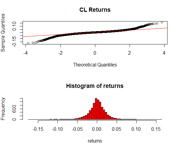
As an exploratory task, we will use the futures prices of WTI Crude Oil and plot the quantiles and the histogram of the returns of the Last field column on the CME_CL_Data_ dataframe. We downloaded this data in the previous article.

# Compare returns quantiles to quantiles of a normal distribution using the qqnorm and qqline commands that plot the quantiles of the series and a quantiles of a normal distribution as a theoretical line

par(mfrow=c(2, 1))

# Define the returns vector with the values of the returns column from  CME_CL_DATA_ 

returns <- CME_CL_Data_$returns
qqnorm(returns, main="CL Returns")
qqline(returns, col="red")

# Generate a histogram with the returns 

ret_hist <- hist(returns, breaks=50,col='red')

CL returns Quantiles and Histogram

Quantiles and Histogram

Both the qqplot and the histogram show that the future prices for CL contract are far from a normal distribution, as they have fat tails at the right and left sides of the histogram and a deviation from the theoretical quantiles line in the qqplot. The histogram shows leptokurtic shape with fat tails and peaks. 

Plot Daily Returns

Next we will plot the returns along the dates of the historical series to have an overview of the more volatile periods in the CL historical series from Quandl.

# Make a plot with daily returns and show one and two standard deviations lines.

dates <- CME_CL_Data_$date
one_std <- sd(returns,na.rm = TRUE)
two_std <- one_std * 2 
plot(returns ~ dates, type='l',col='blue')
abline(h=c(-one_std,one_std),col='red')
abline(h=c(-two_std,two_std),col='black')

Returns CL Futures 1983- 2019

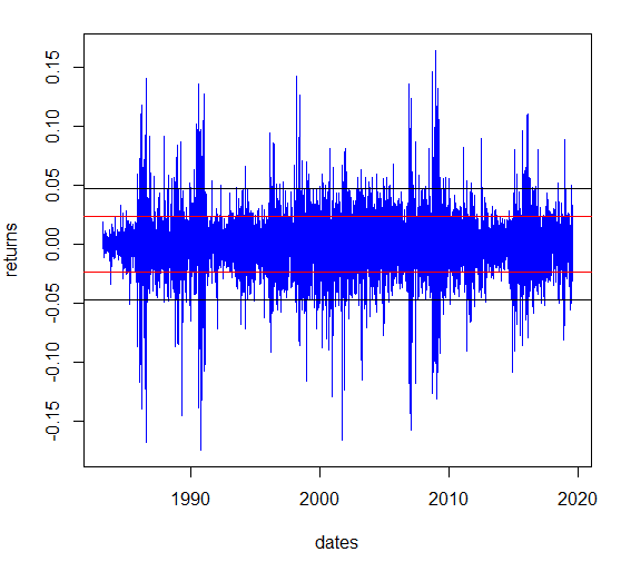
Observing the returns series of the CL futures for the overall period we can detect that the returns expand beyond two standard deviation(black lines) in many periods such as 1991 (Golf War), and 2008 (Oil Crisis).

Futures Prices have High Autocorrelation

In the returns graph, we can also observe that future prices show higher autocorrelation which means that the value of one observation is related to the immediately previous observation. Empirically, this means that negative returns are correlated with future negative returns and positive returns tend to be followed by positive returns.  

This correlation is measured by a decay factor which is a coefficient between 0 and 1 that represents how much the next observation would vary with respect to the previous observation. The autocorrelation formula gives a coefficient to each lag of the original series to weight the persistence of each lag. 

Futures are Suitable for Portfolio Diversification

Another property of future contracts is that they can be used to diversify portfolios. Commodity futures are used by hedge funds and other investment funds as a method to diversify portfolios composed of stocks and bonds. Commodities prices show negative correlation with stocks and bond prices among most time horizons, which convert them in a vehicle to diversify portfolios. Moreover, to satisfy the demand of commodities futures, the Goldman Sachs Commodity Index (GSCI) was created by Goldman Sachs Organization.

Future prices show higher volatility when the contract is approaching its expiration date. The intuition of this hypothesis is based on the fact that when the commodity contract is near expiration, more information is revealed about the commodity and so prices would update based on the new information. At the beginning of the future contract life, little information is known about the future spot price.   

As we have observed above, futures contracts have higher volatility periods along the historical series. Some futures prices such as commodities are affected by the supply and demand of the asset and can show higher volatility for certain periods. 

Plot Volatility by Year

The next analysis provides an overview about the volatility by year of the CL future prices. The following R code would be useful to provide insights about the different volatility periods in CL futures contracts. We will compare the standard deviation values for the last 13 years of the CL continuous historical series from Quandl. 

We will use the CME_CL_Data_ dataframe to create a new dataframe with data for the last 13 years and plot the volatility by year in a bar plot.

# Subset the CME_CL_Data_ to obtain the last 13 years

CME_CL_Vol <- subset(CME_CL_Data_, date > '2007-01-01')

# Create a new column called 'year' with the year of the date column. We use the command substr to extract the required valued by their index position(1 to 4).

CME_CL_Vol$year <- substr(CME_CL_Vol$date,1,4)

# The tapply command calculate the standard deviation of the returns by year.
# Is a useful function to perform calculations between groups. We group the 
# data of the returns by year, passing the returns and the year columns as the first #and  second parameter of tapply, and then pass the sd function in the third #parameter of the function. 

vol_by_year <- tapply(CME_CL_Vol$returns,CME_CL_Vol$year,sd,na.rm=TRUE)
vol_by_year_df <- data.frame(round(vol_by_year,4))
colnames(vol_by_year_df)  <-  'VolByYear'

barplot(vol_by_year, main ='CL Volatility by Year', col=c('grey80',' grey81',' grey82','grey82' ,'grey84', 'grey85','grey86','grey87','grey88','grey89','grey90','grey91','grey92'),las=2)

CL Contract Prices Volatility by Year 2007-2019

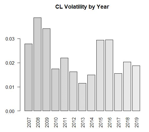
As was expected the highest volatility was in 2008 when the oil prices plummeted after the energy crisis. The effect of the crisis persisted until 2009 where the volatility level was extremely high too. The period between 2015-2016 shows a high level of volatility on CL future prices.