Quantstrat Example in R - RSI Strategy
In this Quantstrat case study, we will create a strategy with the Relative Strength Index (RSI) indicator that gives signals related to overbought and oversold regimes.
RSI Strategy Entry and Exit Signals
In our strategy, we will work with the RSI signal to generate long positions only. We will analyze the strategy with 2 different exit conditions during the whole period.
The first exit condition is when the RSI is greater than 70. In this case we liquidate our long position by selling the asset. This exit point has good effect on some occasions but has the problem that doesn’t prevent for a big fall in prices that could cause high drawdowns on the strategy.
The second exit condition is to add a stop loss. Using a stop loss is more conservative because the price could reach the stop loss and then starts to rise again, but we make sure that our capital will not go down below a certain level defined by the stop loss.
The next step consists of coding the strategy with quantstrat package with the first exit point (RSI threshold exit point), show the performance and risk metrics for this strategy and then run the same strategy with the stop loss order and get the performance and risk metrics. Finally we will compare both results.
Start a new R session and ensure that the quantstrat and ggplot2 libraries are loaded.
Initialize Currency and Instruments
- Initialize current (USD)
- Create symbol variable (we will use the Apple stock - AAPL)
- Set timezone
- Define the stock metadata using the stock() function
1currency('USD')
2
3symbol <- 'AAPL'
4
5Sys.setenv(TZ="UTC")
6
7stock(symbol,currency='USD',multiplier=1)
8
9
Define Dates and Load Historical Data
1# The initDate is used in the initialization of the portfolio and orders objects, and should be less than the startDate, which is the date of the data.
2
3initDate <- '2012-01-10'
4
5startDate <- '2014-01-01'
6
7startEquity <- 100000
8
9endDate <- '2019-08-14'
10
11# Fetch the data from tiingo api. This command require an api key that can be acquired in the tiingo site
12
13# Get your free Tiingo API Token from https://api.tiingo.com/
14
15token <- 'your api key'
16
17getSymbols(symbol,from=startDate,to=endDate,adjust=TRUE,src='tiingo',api.key=token)
18
Initialize Portfolio, Account and Order Objects
1# Name the strategy, portfolio and account with the same name
2
3portName <- stratName <- acctName <- 'AAPLPort'
4
5# Remove objects associated with a strategy
6
7rm.strat(stratName)
8
9# Initialization of the Portfolio, Account and Orders objects with their required parameters. The startEquity value in the initEq parameter on the account initialization is added in order to compute returns.
10
11initPortf(portName,symbols=symbol,initDate = startDate)
12
13initAcct(acctName,portfolios = portName,initDate = startDate,initEq = startEquity)
14
15initOrders(portfolio=portName,startDate=startDate)
16
Initialize and Store the Strategy
1# Initialize and store the strategy
2
3strategy(stratName,store=TRUE)
4
Add Indicators
1# Define RSI Indicator
2
3add.indicator(strategy=stratName, name="RSI", arguments=list(price = quote(Cl(mktdata)), maType="EMA"), label="RSI")
4
5# The applyIndicators function allow to observe the indicators for a specific symbol while making progress in building the strategy
6
7test <- applyIndicators(stratName, mktdata=OHLC(AAPL))
8
9tail(test,10)
10
11           AAPL.Open AAPL.High AAPL.Low AAPL.Close  rsi.RSI
122019-08-01  213.0837  217.1979 205.9545   207.6345 53.73663
132019-08-02  204.7456  205.6422 200.8605   203.2414 41.63635
142019-08-05  197.2344  197.8909 191.8450   192.6021 25.55593
152019-08-06  195.5608  197.3111 193.2995   196.2482 35.41851
162019-08-07  194.6642  198.7984 193.0803   198.2804 40.48905
172019-08-08  199.4360  202.7532 198.6290   202.6536 50.19806
182019-08-09  201.3000  202.7600 199.2900   200.9900 46.84356
192019-08-12  199.6200  202.0516 199.1500   200.4800 45.76186
202019-08-13  201.0200  212.1400 200.8300   208.9700 62.42724
212019-08-14  203.1600  206.4400 202.5869   202.7500 49.55560
22
Add Signals
We will add the signals for entry and exit. The RSI signal to generate long positions when RSI crosses 30, and the exit signal when reaches 70.
1add.signal(strategy = stratName, name="sigThreshold",
2           arguments = list(threshold=30, 		column="RSI",relationship="lt",cross =TRUE),label="LongEntry")
3
4add.signal(strategy = stratName, name="sigThreshold",
5           arguments = list(threshold=70, column="RSI",relationship="gt",cross =TRUE),label="LongExit")
6
7# With applySignal(), it is possible to observe the signal columns as well as the remaining information of the mktdata object.
8
9sig <- applySignals(stratName,mktdata)
10
11          AAPL.Open AAPL.High AAPL.Low AAPL.Close  rsi.RSI LongEntry LongExit
122019-08-01  213.0837  217.1979 205.9545   207.6345 53.73663         0        0
132019-08-02  204.7456  205.6422 200.8605   203.2414 41.63635         0        0
142019-08-05  197.2344  197.8909 191.8450   192.6021 25.55593         1        0
152019-08-06  195.5608  197.3111 193.2995   196.2482 35.41851         0        0
162019-08-07  194.6642  198.7984 193.0803   198.2804 40.48905         0        0
172019-08-08  199.4360  202.7532 198.6290   202.6536 50.19806         0        0
182019-08-09  201.3000  202.7600 199.2900   200.9900 46.84356         0        0
192019-08-12  199.6200  202.0516 199.1500   200.4800 45.76186         0        0
202019-08-13  201.0200  212.1400 200.8300   208.9700 62.42724         0        0
212019-08-14  203.1600  206.4400 202.5869   202.7500 49.55560         0        0
22
23
Add Strategy Rules
1add.rule(strategy = stratName,name='ruleSignal',
2         arguments = list(sigcol="LongEntry",sigval=TRUE,
3                          orderqty= 100,  ordertype="market", orderside="long",
4                          replace=FALSE),
5         label="longEnter", enabled=TRUE,  type="enter")
6
7
8add.rule(strategy = stratName,name='ruleSignal',
9         arguments = list(sigcol="LongExit",sigval=TRUE,
10                          orderqty= "all",  ordertype="market", orderside="long",
11                          replace=FALSE),
12         label="longExit", enabled=TRUE,  type="exit")
13
14
Apply the Strategy to the Portfolio
We will now apply the strategy to portfolio and then update the portfolio, account and equity.
1# Apply strategy to the portfolio
2
3t1 <- Sys.time()
4
5results <- applyStrategy(stratName,portfolios = portName,symbols = symbol)
6
7t2 <- Sys.time()
8
9print(t2-t1)
10
11# Set up analytics. Update portfolio, account and equity
12
13updatePortf(portName)
14
15dateRange <- time(getPortfolio(portName)$summary)[-1]
16
17updateAcct(portName,dateRange)
18
19updateEndEq(acctName)
20
Portfolio Equity Returns
1tStats <- tradeStats(Portfolios = portName, use="trades", inclZeroDays=FALSE)
2
3# Plot the equity curve of the strategy
4
5final_acct <- getAccount(acctName)
6
7final_acct
8
9options(width=70)
10
11plot(final_acct$summary$End.Eq, main = "RSI Portfolio Equity")
12
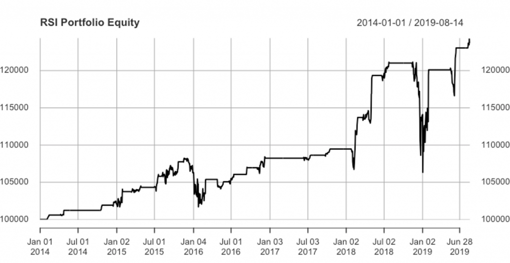
APPL Portfolio Equity returns – First RSI Strategy

The strategy has positive returns in the whole period. However we can observe a huge drawdown at the end of 2018. As we stated in the risk management section, the stop loss prevents high equity losses when market go down as is the case of AAPL stock at the end of 2018.
Let’s see some performance and risk metrics of this strategy.
Strategy Statistics
1tab.profit <- tStats %>%   select(Net.Trading.PL, Gross.Profits, Gross.Losses, Profit.Factor)
2
3t(tab.profit)
4
5                       AAPL
6Net.Trading.PL 23699.883948
7Gross.Profits  27293.575028
8Gross.Losses   -3593.691080
9Profit.Factor      7.594858
10
11tab.wins <- tstats %>%
12  select(Avg.Trade.PL, Avg.Win.Trade, Avg.Losing.Trade, Avg.WinLoss.Ratio)
13
14
15t(tab.wins)
16
17                          AAPL
18Avg.Trade.PL       1184.994197
19Avg.Win.Trade      1605.504413
20Avg.Losing.Trade  -1197.897027
21Avg.WinLoss.Ratio     1.340269
22
23# Note: The pipe operator ( %>% )to select specific columns in a part of the dplyr package.
24
Obtain Risk Metrics
1rets <- PortfReturns(Account = acctName)
2
3rownames(rets) <- NULL
4
5tab.perf <- table.Arbitrary(rets,
6                            metrics=c(
7                              "Return.cumulative",
8                              "Return.annualized",
9                              "SharpeRatio.annualized",
10                              "CalmarRatio"),
11                            metricsNames=c(
12                              "Cumulative Return",
13                              "Annualized Return",
14                              "Annualized Sharpe Ratio",
15                              "Calmar Ratio"))
16tab.perf
17
18                        AAPL.DailyEqPL
19Cumulative Return           0.24846722
20Annualized Return           0.04034198
21Annualized Sharpe Ratio     0.55102551
22Calmar Ratio                0.28209635
23
24tab.risk <- table.Arbitrary(rets,
25                            metrics=c(
26                              "StdDev.annualized",
27                              "maxDrawdown"
28                              ),
29                            metricsNames=c(
30                              "Annualized StdDev",
31                              "Max DrawDown"))
32
33tab.risk
34
35                  AAPL.DailyEqPL
36Annualized StdDev     0.07321255
37Max DrawDown          0.14300782
38
The Maximum Drawdown is 14% of the Equity. This represents a big drawdown and in some circumstances is not acceptable. Some strategies are constrained to have a Maximum Drawdown lower than a threshold. For this reason is important to run the same strategy and observe the stop loss effect to prevent big losses.
RSI Stop Loss Order Exit
We will revise our strategy to add a stop loss signal. This is to prevent large drawdowns.
Initialize Variables and Objects
1.orderqty <- 100
2.txnfees <- -10
3.stoploss <- 0.05 # Stop loss percentage (5%) applied to the fill price of the entry order
4
5symbols <- c('AAPL')
6
7# Name the strategy, portfolio and account with the same name
8
9portName <- stratName <- acctName <- 'AAPLPort'
10
11rm.strat(portName)
12
13rm.strat(acctName)
14
15# For stocks the multiplier is always 1
16
17stock(symbols, currency="USD", multiplier=1)
18
19# Remove objects associated with a strategy
20
21rm.strat(stratName)
22# Initialization of the Portfolio, Account and Orders objects with their required parameters. The startEquity value in the initEq parameter on the account initialization is added in order to compute returns.
23
24initPortf(portName,symbols=symbol,initDate = startDate)
25
26initAcct(acctName,portfolios = portName,initDate =
27startDate,initEq = startEquity)
28
29initOrders(portfolio=portName,startDate=startDate)
30
31# Initialize and store the strategy
32
33strategy(stratName,store=TRUE)
34
Add Strategy Indicators
1# Define RSI Indicator
2
3add.indicator(strategy=stratName, name="RSI", arguments=list(price = quote(Cl(mktdata)), maType="EMA"), label="RSI")
4
5
Add Signals
1# Add Signals
2
3add.signal(strategy = stratName, name="sigThreshold",
4           arguments = list(threshold=30, column="RSI",relationship="lt",cross =TRUE),label="LongEntry")
5
6add.signal(strategy = stratName, name="sigThreshold",
7           arguments = list(threshold=70, column="RSI",relationship="gt",cross =TRUE),label="LongExit")
8
Add Strategy Rules
1add.rule(strategy = stratName,name='ruleSignal',
2         arguments = list(sigcol="LongEntry",sigval=TRUE,
3                          orderqty= 100,  ordertype="market", orderside="long",
4                          replace=FALSE),
5         label="longEnter", enabled=TRUE,  type="enter")
6
7
8add.rule(strategy = stratName,name='ruleSignal',
9         arguments = list(sigcol="LongExit",sigval=TRUE,
10                          orderqty= "all",  ordertype="market", orderside="long",
11                          replace=FALSE),
12         label="longExit", enabled=TRUE,  type="exit")
13
14# This third rule adds the stop loss condition
15
16add.rule(stratName,
17         name = "ruleSignal",
18         arguments = list(sigcol = "LongEntry" ,
19                          sigval = TRUE,
20                          replace = FALSE,
21                          orderside = "long",
22                          ordertype = "stoplimit",
23                          tmult = TRUE,
24                          threshold = quote(.stoploss),
25                          TxnFees = -10,
26                          orderqty = "all"),
27         type = "chain",
28         parent = "longEnter",
29         label = "StopLossLONG",
30         enabled = FALSE)
31
32
With these rules, the exit points can be triggered in two situations. First when the RSI reach the 70 threshold while we are in the market, and secondly when the AAPL price reached the defined stop loss of 5% of the price.
The rule for the stop loss need a threshold parameter with the percentage of the filled price that the stop loss represents, and we should add the “chain” value to the type parameter, and invoke the parent order of the stop loss order which is the longEnter order.
1for(symbol in symbols){
2    addPosLimit(portfolio = portName,
3              symbol = symbol,
4              timestamp = startDate,
5              maxpos = .orderqty)
6}
7
We have defined the stop loss order with the enable parameter set to FALSE, so here we enable the stop loss order:
1enable.rule(stratName,
2            type = "chain",
3            label = "StopLoss")
4
Apply Strategy
1#apply strategy
2
3t1 <- Sys.time()
4results <- applyStrategy(stratName,portfolios = portName,symbols = symbols)
5
6t2 <- Sys.time()
7
8print(t2-t1)
9
10
Update Portfolio, Account and Equity
1#set up analytics
2
3updatePortf(portName)
4
5dateRange <- time(getPortfolio(portName)$summary)[-1]
6
7updateAcct(portName,dateRange)
8
9updateEndEq(acctName)
10
New Performance Metrics
1tStats <- tradeStats(Portfolios = portName, use="trades", inclZeroDays=FALSE)
2
3final_acct <- getAccount(acctName)
4
5options(width=70)
6
7plot(final_acct$summary$End.Eq, main = "RSI Portfolio Equity")
8
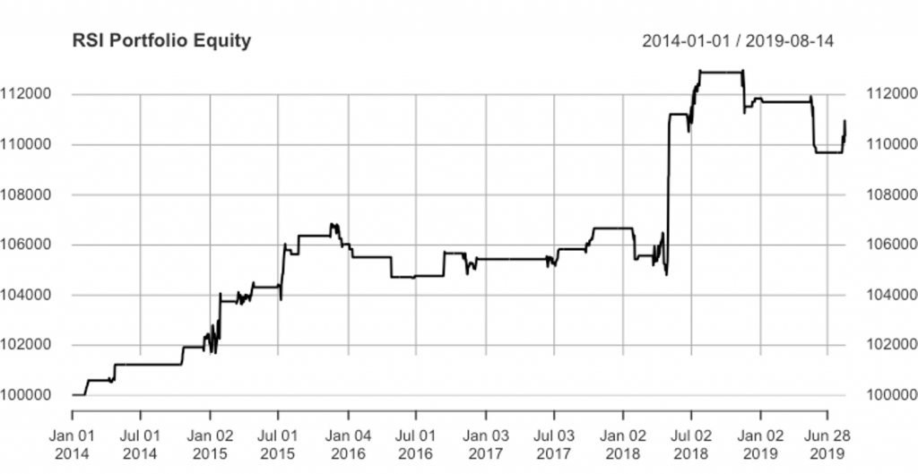
APPL Portfolio Equity returns – Second RSI Strategy

The first impression is while this second strategy has less returns at the end of the period compared to the first strategy, in this case we prevent the strategy from large drawdowns. With the stop loss parametrization we have avoided big losses.
1# Performance and Risk Metrics
2# Profits
3tab.profit <- tStats %>%
4  select(Net.Trading.PL, Gross.Profits, Gross.Losses, Profit.Factor)
5t(tab.profit)
6                       AAPL
7Net.Trading.PL 10340.877309
8Gross.Profits  18134.854581
9Gross.Losses   -7793.977272
10Profit.Factor      2.326778
11
12tab.wins <- tStats %>%
13  select(Avg.Trade.PL, Avg.Win.Trade, Avg.Losing.Trade, Avg.WinLoss.Ratio)
14t(tab.wins)
15
16                         AAPL
17Avg.Trade.PL       304.143450
18Avg.Win.Trade      906.742729
19Avg.Losing.Trade  -556.712662
20Avg.WinLoss.Ratio    1.628745
21
22
23rets <- PortfReturns(Account = acctName)
24rownames(rets) <- NULL
25
26tab.perf <- table.Arbitrary(rets,
27                            metrics=c(
28                              "Return.cumulative",
29                              "Return.annualized",
30                              "SharpeRatio.annualized",
31                              "CalmarRatio"),
32                            metricsNames=c(
33                              "Cumulative Return",
34                              "Annualized Return",
35                              "Annualized Sharpe Ratio",
36                              "Calmar Ratio"))
37tab.perf
38
39                        AAPL.DailyEqPL
40Cumulative Return           0.10713135
41Annualized Return           0.01830312
42Annualized Sharpe Ratio     0.75692880
43Calmar Ratio                0.55756178
44
Risk Statistics
1# Risk Statistics
2
3tab.risk <- table.Arbitrary(rets,
4                            metrics=c(
5                              "StdDev.annualized",
6                              "maxDrawdown"),
7                            metricsNames=c(
8                              "Annualized StdDev",
9                              "Max DrawDown"))
10tab.risk
11
12                  AAPL.DailyEqPL
13Annualized StdDev     0.02418077
14Max DrawDown          0.03282708
15
The Max Drawdown when we set the stop loss in the RSI strategy is 3.28% while in the first RSI strategy (without stop loss), the Max Drawdown was 14%. The RSI strategy without the Stop Loss shows better returns at the end of the period, but when we add a stop loss, we prevent from large losses when market drops and both the Sharpe Ratio and Calmar Ratio improves. To conclude, if our decision about strategy selection, is based on the Sharpe Ratio (like many strategies), we should select the RSI with the stop loss order as it has a higher Sharpe Ratio than the RSI strategy without the stop loss.


