Quantstrat Example in R - EMA Crossover Strategy

EMA refers to Exponential Moving Average. This type of moving average reacts faster to recent price changes than a simple moving average. The 12- and 26-day EMAs are the most popular short-term averages. Exponential Moving Average shows the average value of the underlying data, most often the price of a security, for a given time period, attributing more weight to the latest changes and less to the changes that lie further away.

Note that moving averages do not predict price direction, but define the current direction with a lag (because of basing on past prices). Despite this lag, moving averages help smooth price action and filter out the noise. 

They also form the building blocks for many other technical indicators and overlays, such as Bollinger Bands, MACD and the McClellan Oscillator. 

These moving averages can be used to identify the direction of the trend or define potential support and resistance levels.

Crossovers

Crossovers are one of the main moving average strategies. A crossover is a signal of a trend reversal is when one moving average crosses another. Two moving averages can be used together to generate crossover signals. 

• The two series chosen are such that one has relatively short moving average and the other has relatively long moving average. 5-day EMA and 35-day EMA would be deemed short-term, while a system using a 50-day SMA and 200-day SMA would be  long-term.
• A bullish crossover occurs when the shorter moving average crosses above the longer moving average. This is also known as a golden cross. 
• A bearish crossover occurs when the shorter moving average crosses below the longer moving average. This is known as a dead cross.

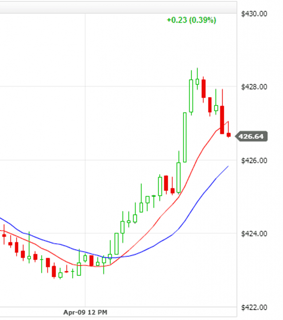
In the below chart, the red line represents the 10-period moving average and the blueline represents the 20-period moving average. Notice how the short-term average crossing the long-term average signals the beginning of an uptrend.

To start building our EMA Crossover strategy, we will first define some variables that the strategy will use, as well as get the historical data for the symbol.  

We will use the QQQ ETF that tracks the Nasdaq 100 Index, as the instrument and over it we will overlay 10-period EMA and 30-period EMA to observe the crossover.

Load the Quantstrat Package in R

1#Load quantstrat in your R environment.
2 
3library(quantstrat) 
4
5# The search command lists all attached packages.
6search()
7

Loading quantstrat causes these other libraries to be loaded automatically: 

• blotter 
• foreach 
• quantmod 
• PerformanceAnalytics 
• FinancialInstrument 
• Defaults 
• TTR 
• xts 
• zoo

Initialize Currency and Instruments

First, we specify the symbols and currencies that we are using. Then we define the stock metadata using the stock() function from the FinancialInstrument package.

1symbolstring <- 'QQQ'
2 
3currency('USD')
4 
5stock(symbolstring,currency='USD',multiplier=1)
6

The FinancialInstrument's functions build and manipulate objects that are stored in an environment named ".instrument" at the top level of the package (i.e. "FinancialInstrument:::.instrument") rather than the global environment. 

You can see what you’ve created in this environment using the ls() function as shown below:

1# Currency and trading instrument objects stored in the 
2# .instrument environment
3 
4ls(envir=FinancialInstrument:::.instrument)
5 
6[1] "QQQ" "USD"
7 
8# blotter functions used for instrument initialization 
9# quantstrat creates a private storage area called .strategy
10 
11ls(all=T)
12 
13[1] ".blotter"     ".strategy" 
14

Load Historical Data

We will now load the historical data. We need to create three date variables: initialization date, start date and end date. We also set the initial equity and also set the timezone.

1# The initDate should be lower than the startDate. The initDate will be used later while initializing the strategy.
2 
3initDate <- '2010-01-01'
4 
5startDate <- '2011-01-01'
6 
7endDate <- '2019-08-10'
8 
9init_equity <- 50000
10 
11 
12# Set UTC TIME
13 
14Sys.setenv(TZ="UTC")
15

The initDate variable needs a date that must occur before the start of data in a backtest. If this isn’t the case, the portfolio will demonstrate a massive drawdown on the initialization date, and many of the backtest statistics will be misleading or nonsensical.

The startDate and endDate variables are endpoints on the data that we will use to fetch for the symbol from yahoo.

We can now fetch the data using the getSymbols() function.

1getSymbols(symbolstring,from=startDate,to=endDate,adjust=TRUE,src='yahoo')
2

Initialize Portfolio and Account

In quantstrat, we need to understand three main concepts: 1) Account, 2) Portfolio, and 3) Strategy.

An account may contain one more multiple portfolios. And each portfolio may contain one more multiple strategies. You can look at it this way:

Account -> Portfolio -> Strategy

In the quantstrat backtesting infrastructure, each strategy runs on a specific portfolio and account. These elements need to be defined and initialized in order to build and backtest a strategy. At first we need to assign names to the strategy, portfolio and account variables. These names could be any string names to identify these elements. We will use the name ‘FirstPortfolio’ for portfolio name, account name, as well as strategy name.

1# Define names for portfolio, account and strategy. 
2 
3portfolioName <- accountName <- strategyName <- "FirstPortfolio"
4 
5# The function rm.strat removes any strategy, portfolio, account, or order book object with the given name. This is important
6 
7rm.strat(strategyName)
8

Once we have the strategy, portfolio and account names, we need to initialize and create objects for the portfolio and the account. These objects would hold the backtesting results as well as the positions, transactions and other aggregate variables of the backtesting. 

Initialization means to create the objects in the context of the Quantstrat package. For this purpose, it is necessary to provide the correct parameters for each of these objects. botter functions are used for portfolio and account initialization.

Initialize Portfolio

To create the portfolio object, we need to provide the portfolio name, stocks symbols or instruments that the portfolio will contain and the initialization date of the backtesting.

We use the following function to construct and initialize a portfolio object:

1initPort(name=..., symbols,, initDate=...)
2 
3# name: is the string name of the portfolio
4 
5# symbols: tickers that the portfolio store
6 
7# initDate: initial data of the backtesting. Should be prior to 
8 
9# the date of the loaded prices.
10

Initialize Account

After we create the portfolio object, we need to define the account object. The account can be related to one or more than one portfolios. 

We use the following function to construct and initialize the account object:

1initAcct(name=..., portfolios, initDate=..., initEq=...)
2 
3# name: is a string that identifies the account name
4 
5# portfolios: is a character vector of strings with the names of the portfolios included in the account, With this parameter we link the portfolio or portfolios to a specific account
6 
7# initDate: is the initial date of the backtesting and requires a date prior to the first close price given. This date will be the date that counts for the initial account equity and initial position
8 
9# initEq: is the initial equity of the portfolio.
10

Both the portfolio and account are initialized below:

1initPortf(name = portfolioName,
2          symbols = symbolstring,
3          initDate = initDate)
4 
5initAcct(name = accountName,
6         portfolios = portfolioName,
7         initDate = initDate,
8         initEq = init_equity)
9 
10

Initialize Order and Strategy

We will now initialize the account object. The function initOrders sets up an order container (order book) for the portfolio. This is a quantstrat specific initialization.

You can check the parameters of initOrders function using the args(initOrders) command. 

1initOrders(portfolio = portfolioName,
2           symbols = symbolstring,
3           initDate = initDate)
4

You can check that the order book is initialized successfully using the get.orderbook(portfolioName) command.

Finally, the strategy object is created with the following code:

1strategy(name, assets, constrains, store)
2 
3# name: the string name of the strategy
4 
5# assets: optional list of assets to apply the strategy to.  
6 
7# Normally these are defined in the portfolio object
8 
9# contstrains: optional portfolio constraints
10 
11# store: can be True or False. If True store the strategy in the environment. Default is False
12

We create the strategy object below. The strategy name should be passed as the first parameter when we generate the indicators, signals and rules of the strategy in order to link all these elements to the strategy defined. 

View Created Objects

Let’s ensure that all the objects are created successfully. We should have the portfolio, account, orderbook and strategy objects.

1ls(all=T)
2 [1] ".blotter"	".strategy"	"accountName"   
3 [4] "endDate"	"init_equity"	"initDate"
4 [7] "portfolioName"	"startDate"	"strategyName"         
5 [10] "symbolstring"  
6 
7# .blotter holds the portfolio and account object 
8  
9ls(.blotter)
10[1] "account.FirstPortfolio"   "portfolio.FirstPortfolio"
11 
12# .strategy holds the orderbook and strategy object
13 
14ls(.strategy)
15[1] "FirstPortfolio"            "order_book.FirstPortfolio"
16

Adding Indicators

Once we have initialized the objects, the next step is to create the indicators that the strategy would use. For this purpose, quantstrat has a full list of technical indicators which are calculated from the market data of the symbol that is loaded in the environment.

The indicators are path independent, which means that they do not depend on account / portfolio characteristics, current positions, or trades. 

Since we are creating an EMA crossover strategy, we will add two indicators: 10-period EMA and 30-period EMA

In quantstrat, we use the add.indicator() function to add indicators. The parameters of the add.indicator() function are: strategy, name, arguments and label.  strategy is the string name of the strategy (defined in the Initialization step) to add the indicator to; name is the indicator function which in this case is “EMA”, but could be RSI, MACD, etc. The arguments parameter has a list with the required inputs to calculate the indicator passed in the name argument. 

1add.indicator(strategy = strategyName, 
2              name = "EMA", 
3              arguments = list(x = quote(Cl(mktdata)), 
4                               n = 10), label = "nFast")
5 
6add.indicator(strategy = strategyName, 
7              name = "EMA", 
8              arguments = list(x = quote(Cl(mktdata)), 
9                               n = 30), 
10              label = "nSlow")
11

Our strategy should now have two indicators. You can confirm this by executing this function: summary(getStrategy(strategyName)).

When we calculate an Exponential Moving Average we need the close price and the lookback period n for the calculation. Observe that we use the mktdata object to get the close prices. This is different from the common procedure in R to retrieve closes price column of a dataframe with the “$” character (dataframe$Close).

mktdata is an internal object that has OHLCV information loaded in the environment (when we get the data using getSymbols), and every time we add an indicator or a signal, a new column is generated in the mktdata object. The label argument would be the column name in the mktdata object with the indicator values. Both signals and indicators are created in a vectorized form and just as indicators, signals are path independent too.

Adding Signals

The next step is to add signals which are generated from the interaction of indicators and market data. Examples include the point at which the fast Moving Average and the slow Moving Average cross each other (or in other cases when the RSI or MACD are greater than or lower than a defined threshold).

In this example we generate a long trade when the fast EMA (10-period EMA) crosses up the slow EMA (30-period EMA), and a short trade when the fast EMA cross down the slow EMA.

In quantstrat, a signal is added using the add.signal() function which takes the following form:

The important parameters are strategy, name, arguments and label.  

strategy: This is the strategy name that we define in the Initialization step. In our example it is stored in the variable strategyName.

name: The name parameter accepts built-in functions that specify the signal type (crossovers, threshold, etc.). It is also possible to create custom functions. We should pass the string name of the function as the parameter value.  Quantstrat has the following built in functions to generate signals: sigComparison, sigCrossover, sigFormula, sigPeak, sigThreshold.  

arguments: These are the arguments to be passed to the indicator function

label: When we create indicators and signals, we must pass a label parameter. In quantstrat labels are logical links between indicators, signals and rules, so is important to create smart labels with an appropriate name of indicators and signals. 

The logic of the signals above is given by the combination of the function on the name parameter, and the arguments parameter that has a list containing the mktdata columns (for the indicators), and the relationship(("gt", "lt", "eq", "gte", "lte") that these columns should hold for creating the new signal in a specific moment of time.

A crossover signal is created using the sigCrossover() function.

Below is the specific code to generate these signals:

1# Add long signal when the fast EMA crosses over slow EMA.
2 
3add.signal(strategy = strategyName,
4           name="sigCrossover",
5           arguments = list(columns = c("nFast", "nSlow"),
6                            relationship = "gte"),
7           label = "longSignal")
8 
9# Add short signal when the fast EMA goes below slow EMA.
10 
11add.signal(strategy = strategyName, 
12           name = "sigCrossover",
13           arguments = list(columns = c("nFast", "nSlow"),
14                            relationship = "lt"),
15           label = "shortSignal")
16

The first signal indicates that a new column labeled longSignal will be created in the mktdata object. The value of longSignal would be true or have the value of 1 when the nFast column (fast EMA)  is greater or equal (“gte”) than the nSlow column (slow EMA). Every time that fast EMA crosses up the slow EMA, the longSignal column will have the value of 1.

The second signal means that the shortSignal column will have the value of 1 when the nFast column (fast EMA)  crosses below (“lt”) the nSlow (slow EMA) column. Every time the fast EMA crosses below the slow EMA, the shortSignal will have the value of 1 and in other case it would have a value of 0. 

Is important to indicate that if we use the sigCrossover function for the signal generation, both columns (shortSignal and longSignal) would have a value of 1 only when the fast EMA crosses up or down the slow EMA. However, if  we use the sigComparison function, the columns longSignal and shortSignal are 1 every time the fast EMA is higher than the slow EMA (for long signal) or every time the fast EMA is lower than the slow EMA (for the slow signal). 

To get the crossover behavior while using the sigComparison function, we can add the parameter Cross = True within the list of the arguments parameter. 

The built-in functions are explained in some more details below:

The sigComparison function compares two columns on the mktdata object, and will return TRUE (1) as long as the specified relationship comparing the first column to the second column (passed as parameters) holds.

The sigCrossover is similar to the above function but only returns TRUE on the timestamp (bar) that the relationship moves from FALSE to TRUE. In the EMA crossover setup, the sigCrossover is only TRUE in the crossover, while the sigComparison is TRUE as long as the condition is achieved.

sigThreshold uses a threshold value to be compared with the indicator. This is useful when we generate signals with indicators based on threshold values such as RSI, MACD, and other oscillators. When the indicator crosses a certain value (threshold) the function returns TRUE .

sigFormula apply a formula to multiple variables. With this function, signals can be generated by chaining conditions with the amp character “&” or evaluate that any of both conditions are True with the “|” character. 

sigPeak identifies local minima or maxima of an indicator (peak/valley signals).

Adding Rules

After indicators and signals are created, the next important step is the generation of the strategy rules. Rules use market data, indicators, signals, and current account / portfolio properties to generate orders. The strategy rules are path dependent because they are related with the portfolio, and with the orders and risk management of the strategy. 

It is not common to send naïve orders, so the rules have to interact with the portfolio and previous orders, to enable different trade sizes and manage risk with different order types. The package provides functionality to simulate and optimize order types. 

In quantstrat, the add.rule() function is used to generate rules and determines the positions we take based on our signals, the types of orders we place, the trade size, and transactions cost of the broker. Overall, the rules allow functionality to enter positions (long and short) and to exit positions (long and short).

The following rule creates a long order to buy 100 shares when the value of the longSignal column in the mktdata object is TRUE.

1# go long when 10-period EMA (nFast) >= 30-period EMA (nSlow)
2 
3add.rule(strategyName,
4         name= "ruleSignal",
5         arguments=list(sigcol="longSignal",
6                        sigval=TRUE,
7                        orderqty=100,
8                        ordertype="market",
9                        orderside="long",
10                        replace = TRUE, 
11                        TxnFees = -10),
12         type="enter",
13         label="EnterLong") 
14

The above rule establishes that when the longSignal column on the mktdata object is TRUE, the strategy will send a market order with an order quantity of 100. 

Rules have just one function in the name parameter which is called “ruleSignal”. Even though the add.rule() has only the ruleSignal function, this function has many different arguments that can take in one of several values. We can customize many features with the add.rule() functions, such as the trade size, the preferred price (open, high, close, low) to trigger and order, transactions fees, stop loss and take profit among others.

The ordertype parameter specifies the type of the order (market, limit, stop loss, stop limit, trailing stop). The replace command tells that this order would replace any open order if it is equal to TRUE. The above rule would create a new column in the mktdata object called EnterLong.

The following rule creates a short order to sell 100 shares when the value of the shortSignal column on the mktdata object is TRUE.

1# go short when 10-period EMA (nFast) < 30-period EMA (nSlow)
2 
3add.rule(strategyName, 
4         name = "ruleSignal", 
5         arguments = list(sigcol = "shortSignal", 
6                          sigval = TRUE, 
7                          orderside = "short", 
8                          ordertype = "market", 
9                          orderqty = -100, 
10                          TxnFees = -10,                     
11                          replace = TRUE), 
12         type = "enter", 
13         label = "EnterShort")
14 
15

Next we should define rules to close both long and short positions. To close a long position we should use the shortSignal column of the mktdata object and pass the order information in the add.rule() function:

1# Close long positions when the shortSignal column is True
2 
3add.rule(strategyName, 
4         name = "ruleSignal", 
5         arguments = list(sigcol = "shortSignal", 
6                          sigval = TRUE, 
7                          orderside = "long", 
8                          ordertype = "market", 
9                          orderqty = "all", 
10                          TxnFees = -10, 
11                          replace = TRUE), 
12         type = "exit", 
13         label = "ExitLong")
14

In the rule, we should always specify the ordertype, orderside, orderqty and the sigcol (column name) in which the rule is created. The orderside can be long or short, ordertype in this case simulates a market order (quantstrat supports different order types).

In quantstrat, market orders are executed at the next bar after receiving the signal. This can cause some gaps with daily data, as the signal is generated in the current bar, and the order bar is the next bar of the signal. However with intraday data, the open of the next bar should be very similar to the close of the current bar. When using monthly data, quantstrat uses current bar execution. 

In the rule above we pass the “exit” value to the type parameter to specify that this order is to exit a current position. We label the rule with the “ExitLong” string, and the orderside is “long” because this order is to close a long position.

The orderside parameter is very important to maintain coherence in the order process.  We should group with "long" those orders which are for buy and sell a long position. And we should group with “short” in the orderside parameter, those orders which are placed to enter and liquidate a short position.

This scheme separates rule executions, such that long sells (orders that are placed to close a long position) won’t work on short positions and vice versa.

The orderqty parameter can be a flat value like 100 shares or 50 shares, but when the order size has a custom function (OsFUN different from Null), the orderqty parameter doesn’t apply. 

The type argument generally has the value “enter” and “exit”. There are other rules types such as “chain” for stop loss orders. When the rule type is “exit”, the string “all” in the orderqty parameter, means to liquidate the position. 

The label argument in the add.rules() can be used for deeper analysis and sometimes is not used because the rule contain the last point of the strategy logic. 

Below, we create the rule for closing a short position has the orderside “short” and is triggered when the longSignal column is TRUE. 

1# Close Short positions when the longSignal column is True
2 
3add.rule(strategyName, 
4         name = "ruleSignal", 
5         arguments = list(sigcol = "longSignal", 
6                          sigval = TRUE, 
7                          orderside = "short", 
8                          ordertype = "market", 
9                          orderqty = "all", 
10                          TxnFees = -10, 
11                          replace = TRUE), 
12         type = "exit", 
13         label = "ExitShort")
14

View Strategy Object

We have now created everything required for our strategy. The strategy object now contains a complete set of quantitative trading rules ready to be applied to a portfolio.

We can review the strategy using the getStrategy and summary command.

1summary(getStrategy(strategyName))
2
3# Summary results are produced below
4
5            Length Class  Mode     
6name        1      -none- character
7assets      0      -none- NULL     
8indicators  2      -none- list     
9signals     2      -none- list     
10rules       3      -none- list     
11constraints 0      -none- NULL     
12init        0      -none- list     
13wrapup      0      -none- list     
14trials      1      -none- numeric  
15call        3      -none- call
16

Apply Strategy to Portfolio

To run the strategy we should use the applyStrategy() method. The applyStrategy function applies the strategy to arbitrary market data. The function takes three main arguments:

• strategy: an object of type ’strategy’ 
• portfolios: a list of portfolios to apply the strategy to 
• symbols: the symbol of the instrument

For this example we pass the strategy and portfolio names, and the symbol that is loaded in the environment.

Calling the applyStrategy generates transactions in the specified portfolio.

1results <- applyStrategy(strategy= strategyName, portfolios = portfolioName,symbols=symbolstring)
2 
3# The applyStrategy() outputs all transactions(from the oldest to recent transactions)that the strategy sends. The first few rows of the applyStrategy() output are shown below
4 
5[1] "2014-03-27 00:00:00 QQQ -100 @ 86.879997"
6[1] "2014-05-14 00:00:00 QQQ 100 @ 87.830002"
7[1] "2014-10-03 00:00:00 QQQ -100 @ 98.169998"
8[1] "2014-10-29 00:00:00 QQQ 100 @ 99.809998"
9[1] "2015-01-07 00:00:00 QQQ -100 @ 101.360001"
10[1] "2015-01-27 00:00:00 QQQ 100 @ 101.440002"
11[1] "2015-01-28 00:00:00 QQQ -100 @ 100.919998"
12[1] "2015-02-06 00:00:00 QQQ 100 @ 103.129997"
13[1] "2015-04-01 00:00:00 QQQ -100 @ 105.050003"
14[1] "2015-04-13 00:00:00 QQQ 100 @ 107.480003"
15[1] "2015-06-16 00:00:00 QQQ -100 @ 108.800003"
16 
17

You can view the transactions table using the getTxns() function.

1getTxns(Portfolio=portfolioName, Symbol=symbolstring)
2 
3           Txn.Qty Txn.Price Txn.Fees Txn.Value Txn.Avg.Cost Net.Txn.Realized.PL
42010-01-01       0      0.00        0         0         0.00              0.0000
52014-03-27    -100     86.88      -10     -8688        86.88            -10.0000
62014-05-14     100     87.83      -10      8783        87.83           -105.0005
72014-10-03    -100     98.17      -10     -9817        98.17            -10.0000
82014-10-29     100     99.81      -10      9981        99.81           -174.0000
92015-01-07    -100    101.36      -10    -10136       101.36            -10.0000
102015-01-27     100    101.44      -10     10144       101.44            -18.0001
112015-01-28    -100    100.92      -10    -10092       100.92            -10.0000
122015-02-06     100    103.13      -10     10313       103.13           -230.9999
132015-04-01    -100    105.05      -10    -10505       105.05            -10.0000
142015-04-13     100    107.48      -10     10748       107.48           -253.0000
152015-06-16    -100    108.80      -10    -10880       108.80            -10.0000
162015-06-19     100    109.89      -10     10989       109.89           -118.9996
172015-06-30    -100    107.07      -10    -10707       107.07            -10.0000
182015-07-17     100    113.59      -10     11359       113.59           -661.9996
192015-08-21    -100    102.40      -10    -10240       102.40            -10.0000
202015-10-13     100    106.10      -10     10610       106.10           -379.9996
212015-12-21    -100    111.05      -10    -11105       111.05            -10.0000
222015-12-30     100    113.27      -10     11327       113.27           -231.9994
232016-01-05    -100    109.31      -10    -10931       109.31            -10.0000
242016-03-02     100    105.83      -10     10583       105.83            337.9996
252016-05-02    -100    106.72      -10    -10672       106.72            -10.0000
262016-05-27     100    110.13      -10     11013       110.13           -350.9996
272016-06-20    -100    107.16      -10    -10716       107.16            -10.0000
282016-07-11     100    110.93      -10     11093       110.93           -386.9996
292016-11-02    -100    115.18      -10    -11518       115.18            -10.0000
302016-11-22     100    118.90      -10     11890       118.90           -382.0002
312016-12-05    -100    116.60      -10    -11660       116.60            -10.0000
322016-12-08     100    118.57      -10     11857       118.57           -207.0002
332017-07-03    -100    136.19      -10    -13619       136.19            -10.0000
342017-07-14     100    142.12      -10     14212       142.12           -602.9993
352017-08-28    -100    142.41      -10    -14241       142.41            -10.0000
362017-08-30     100    144.65      -10     14465       144.65           -233.9990
372018-02-09    -100    156.10      -10    -15610       156.10            -10.0000
382018-02-21     100    164.82      -10     16482       164.82           -882.0001
392018-03-26    -100    164.40      -10    -16440       164.40            -10.0000
402018-04-20     100    162.30      -10     16230       162.30            199.9991
412018-04-23    -100    161.89      -10    -16189       161.89            -10.0000
422018-05-08     100    166.07      -10     16607       166.07           -428.0008
432018-10-09    -100    179.63      -10    -17963       179.63            -10.0000
442019-01-17     100    163.63      -10     16363       163.63           1590.0000
452019-05-15    -100    183.09      -10    -18309       183.09            -10.0000
462019-06-17     100    183.74      -10     18374       183.74            -75.0009
47 
48

Executing the applyStrategy also creates a special variable called mktdata. It is a time series object which contains the historic price data as well as the calculated indicators, signals, and rules. It is helpful to look at what the mktdata object contains.

1mktdata["2019"]
2 
3           QQQ.Open QQQ.High QQQ.Low QQQ.Close QQQ.Volume QQQ.Adjusted EMA.nFast EMA.nSlow longSignal shortSignal
42019-01-02   150.99   155.75  150.88    154.88   58576700     154.2576  154.0980  159.4152         NA          NA
52019-01-03   152.60   153.26  149.49    149.82   74820200     149.2179  153.3202  158.7962         NA          NA
62019-01-04   152.34   157.00  151.74    156.23   74709300     155.6022  153.8492  158.6306         NA          NA
72019-01-07   156.62   158.86  156.11    158.09   52059300     157.4547  154.6203  158.5957         NA          NA
82019-01-08   159.54   160.11  157.20    159.52   49388700     158.8789  155.5111  158.6554         NA          NA
92019-01-09   160.14   161.52  159.47    160.82   46491700     160.1737  156.4764  158.7950         NA          NA
102019-01-10   159.60   161.37  158.70    161.28   38943400     160.6319  157.3498  158.9553         NA          NA
112019-01-11   160.33   160.86  159.79    160.69   30176600     160.0442  157.9571  159.0672         NA          NA
122019-01-14   159.33   159.96  158.59    159.27   30710200     158.6299  158.1958  159.0803         NA          NA
132019-01-15   160.00   162.60  159.91    162.38   40874200     161.7274  158.9566  159.2932         NA          NA
142019-01-16   162.65   163.78  162.29    162.35   33812200     161.6976  159.5736  159.4904          1          NA
152019-01-17   161.83   164.36  161.57    163.63   39329000     162.9724  160.3111  159.7575         NA          NA
162019-01-18   164.78   166.02  163.82    165.25   57183200     164.5859  161.2091  160.1118         NA          NA
172019-01-22   164.06   164.14  160.76    161.94   56711700     161.2892  161.3420  160.2298         NA          NA
182019-01-23   162.77   163.51  160.32    162.15   38106100     161.4984  161.4889  160.3537         NA          NA
192019-01-24   162.68   163.44  162.06    163.20   32417800     162.5441  161.8000  160.5373         NA          NA
202019-01-25   164.51   165.65  163.95    165.15   36515900     164.4863  162.4091  160.8349         NA          NA
212019-01-28   163.02   163.12  161.75    163.11   33491200     162.4545  162.5365  160.9817         NA          NA
222019-01-29   163.20   163.24  160.99    161.57   30784200     160.9207  162.3608  161.0196         NA          NA
232019-01-30   163.40   166.28  162.89    165.68   41346500     165.0142  162.9643  161.3203         NA          NA
242019-01-31   166.70   168.99  166.47    168.16   37258400     167.4842  163.9090  161.7616         NA          NA
25 
26

Update Portfolio, Account and Equity

After executing the strategy, we should update the portfolio, account and the final equity for the account. 

1updatePortf(portfolioName)
2 
3dateRange <- time(getPortfolio(portfolioName)$summary)[-1]
4 
5updateAcct(portfolioName,dateRange)
6 
7updateEndEq(accountName)
8 
9

updatePortf() calculates the Profit & Loss for each symbol in symbols.

updateAcct() calculates the equity from the portfolio data. 

updateEndEq() updates the ending equity for the account. 

The three functions must be called in order.