Quantstrat - EMA Crossover Strategy - Performance and Risk Metrics
Once we have the strategy results, quantstrat provides many functions to analyze the strategy and observe important metrics of performance and risk. We would combine the quantstrat package with the PerformanceAnalytics package to show important performance and risk metrics in a trading strategy. We will look at the following:
- Plot the Strategy Performance
- Strategy Statistics and Stats per Trade
- Portfolio Returns
- Account Summary and Equity Curve
- Portfolio Summary and Strategy Performance
- Equity Return Distribution
Plot the Strategy Performance
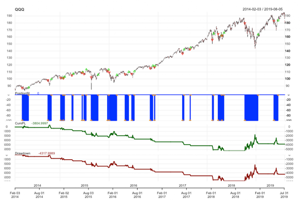
We can plot the performance using the chart.Posn(). The chart.Posn() takes two parameters that are portfolio name and the symbol string and return a chart with the symbol price series, the accumulated profit loss and the Drawdown charts. The trades of the strategy are marked in green and red on the price series chart.
1# Chart Performance of the Strategy
2
3chart.Posn(portfolioName, Symbol = symbolstring)
4
5
QQQ EMA Crossover Prices, Strategy P&L and Drawdowns
Strategy Statistics
tradeStats() function calculates statistics about the strategy. These statistics are related to measures about the strategy profits, risk metrics and general features of the strategy such as number of transactions, highest profitable trade, highest loser trade, average profit per trade among others. In our example, we have the following information:
1tstats <- tradeStats(portfolioName)
2
3tstats <- data.frame(t(tstats))
4
5colnames(tstats)
6
7tstats
8
9                              QQQ
10Portfolio          FirstPortfolio
11Symbol                        QQQ
12Num.Txns                       42
13Num.Trades                     21
14Net.Trading.PL              -3805
15Avg.Trade.PL            -171.1905
16Med.Trade.PL            -231.9994
17Largest.Winner               1590
18Largest.Loser           -882.0001
19Gross.Profits            2127.999
20Gross.Losses            -5722.998
21Std.Dev.Trade.PL         485.9721
22Std.Err.Trade.PL         106.0478
23Percent.Positive         14.28571
24Percent.Negative         85.71429
25Profit.Factor           0.3718328
26Avg.Win.Trade            709.3329
27Med.Win.Trade            337.9996
28Avg.Losing.Trade        -317.9444
29Med.Losing.Trade        -243.4995
30Avg.Daily.PL            -171.1905
31Med.Daily.PL            -231.9994
32Std.Dev.Daily.PL         485.9721
33Std.Err.Daily.PL         106.0478
34Ann.Sharpe              -5.592018
35Max.Drawdown            -5822.998
36Profit.To.Max.Draw     -0.6534434
37Avg.WinLoss.Ratio        2.230997
38Med.WinLoss.Ratio        1.388092
39Max.Equity               512.9992
40Min.Equity              -5309.999
41End.Equity                  -380
42
The perTradeStats() function takes two arguments that are the portfolio name and the symbols strings and outputs the statistics and results by trade. The results contain information such as: the net profit for each trade, the start and end time of each trade, the percentage of profit of the trade, among other interesting variables. We will not show the output of this function, but feel free to try it in R Studio.
Portfolio Returns
The PortfReturns(account) show the daily returns for each symbol of the strategy. We would pass the output of the PortReturns() to the table.Arbitrary function of the PerformanceAnalytics package to condense and create fundamental metrics with the returns of the strategy.
1# Store the returns of the strategy in an object called rets
2
3rets <- PortfReturns(Account = accountName)
4
5rownames(rets) <- NULL
6
7tab.perf <- table.Arbitrary(rets,
8 metrics=c(
9 "Return.cumulative",
10 "Return.annualized",
11 "SharpeRatio.annualized",
12 "CalmarRatio"),
13 metricsNames=c(
14 "Cumulative Return",
15 "Annualized Return",
16 "Annualized Sharpe Ratio",
17 "Calmar Ratio"))
18
19tab.perf #displays the performance metrics
20
21 QQQ.DailyEqPL
22Cumulative Return -0.07613984
23Annualized Return -0.01429584
24Annualized Sharpe Ratio -0.42604174
25Calmar Ratio -0.12881185
26
27
28tab.risk <- table.Arbitrary(rets,
29 metrics=c(
30 "StdDev.annualized",
31 "maxDrawdown",
32 "VaR",
33 "ES"),
34 metricsNames=c(
35 "Annualized StdDev",
36 "Max DrawDown",
37 "Value-at-Risk",
38 "Conditional VaR"))
39
40tab.risk #displays the risk metrics
41
42 QQQ.DailyEqPL
43Annualized StdDev 0.03355503
44Max DrawDown 0.11098234
45Value-at-Risk -0.00248965
46Conditional VaR -0.00248965
47
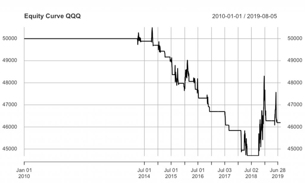
48Account Summary and Equity Curve
The getAccount(AccountName) function returns the account summary and equity curve of the strategy.
1a <- getAccount(accountName)
2
3equity <- a$summary$End.Eq
4
5plot(equity, main = "Equity Curve QQQ")
6
Equity Curve QQQ EMA Crossover Strategy
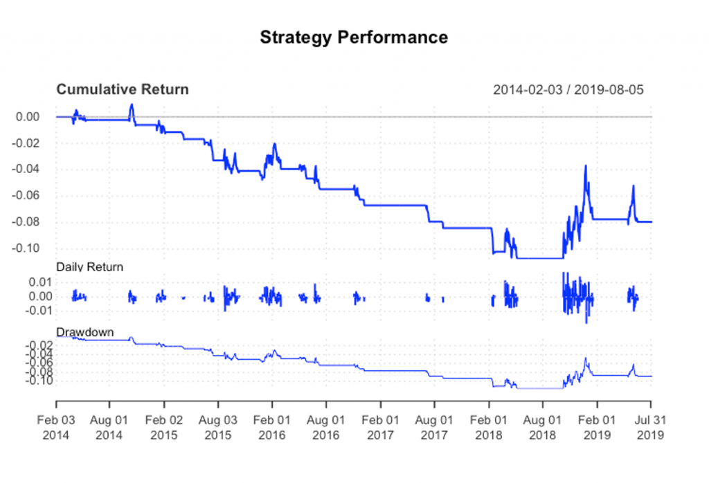
Portfolio Summary and Strategy Performance
The getPortfolio(portfolioName) function returns the portfolio summary. With this function we can view how the portfolio object is updated on a daily basis every time we have new transactions.
1portfolio <- getPortfolio(portfolioName)
2
3portfolioSummary <- portfolio$summary
4
5colnames(portfolio$summary)
6
7"Long.Value"           "Short.Value"          "Net.Value"
8"Gross.Value"          "Period.Realized.PL"   "Period.Unrealized.PL"
9"Gross.Trading.PL"     "Txn.Fees"             "Net.Trading.PL"
10
These are the columns of the portfolioSummary xts object. Every time we have a new transaction these columns would be updated.
1## Account Performance Summary
2
3ret <- Return.calculate(equity, method = "log")
4
5ret
6
7charts.PerformanceSummary(ret, colorset = bluefocus,
8                          main = "Strategy Performance")
9
Cumulative Return, Daily Returns and Drawdown QQQ EMA Crossover Strategy
Equity Returns Distribution
We can also draw a boxplot with the daily equity returns distribution of the strategy.
1rets <- PortfReturns(Account = accountName)
2
3chart.Boxplot(rets, main = "QQQ Returns", colorset= rich10equal)
4
5
Daily Equity Returns Distribution

As we observed, quantstrat provides many tools for the analysis of a trading strategy from multiple perspectives. With these tools we can get accurate information about strategy results and risks. In the next section, we will create a new strategy and with that explore some more features and functionality of quantstrat.
