Quantstrat Case Study - Multiple Symbol Portfolio
One of the main advantages of quantstrat package is that we can backtest strategies with multiple symbols as fast as with one symbol. The package provides fast computations for multiple symbols that allow analysts to get insights of strategies in an efficient approach.
In this case study we will build a strategy that works with 9 ETFs which are described below, and its signal is based on the three Exponential Moving Average (EMA) Crossover in order to run the trend. There are three EMAs that generate a crossover signal to buy when EMA4 > EMA9 > EMA18 and exit positions when EMA4 < EMA9 < EMA18.
In the performance analysis we will get the same info as we did before, but with the breakdown by symbol. This leads to an analysis by symbols where we can get an overview of the worst and best performing symbols. The steps are the same as before: Objects Initialization, Add Indicators, Add Signal, Add Rules, Apply the Strategy to the Portfolio, and Get Metrics.
Before proceeding, start a new R session and ensure that the quantstrat and ggplot2 libraries is loaded.
Note: For convenience, the complete R file is attached below.
Initialize Currency and Instruments
- Initialize current (USD)
- Create symbol variable (we will use the Apple stock - AAPL)
- Set timezone
- Define the stock metadata using the stock() function
1# Make sure quantstrat, dplyr and ggplot2 are loaded before starting.
2# library(quantstrat)
3# library(dplyr)
4# library(ggplot2)
5
6# User search() to check what's loaded
7
8# Initialize the currency. The accounting analytics back-end systems need to know what currency the prices are listed in
9
10currency('USD')
11
12# Set the time to UTC, since that’s the time zone for a “Date” class object. Some orders need the time to be in UTC
13
14Sys.setenv(TZ="UTC")
15
16# Create a Symbols vector
17
18Symbols <- c('SPY',#
19             'IWM', # iShares Russell 2000 ETF
20             'QQQ', # PowerShares QQQ Trust, Series 1
21             'IYR', # iShares U.S. Real Estate ETF
22             'TLT', # iShares 20+ Year Treasury Bond ETF
23             'EEM', # iShares MSCI Emerging Markets ETF
24             'EFA', # iShares MSCI EAFE ETF
25             'GLD', # SPDR Gold Trust
26             'DBC' # Invesco DB Commodity Index
27)
28
29# Define the stock metadata
30
31stock(Symbols,currency='USD',multiplier=1)
32
Define Dates and Load Historical Data
1# The initDate is used in the initialization of the portfolio and orders objects, and should be less than the startDate, which is the date of the data.
2
3initDate <- '2013-01-10'
4
5startDate <- '2014-07-01'
6
7startEquity <- 100000
8
9endDate <- '2019-08-14'
10
11tradeSize <- startEquity/length(symbols)
12
13# Fetch the data from tiingo api. This command require an api key that can be acquired in the tiingo site
14
15token <- token <- 'your api key'
16getSymbols(Symbols,from=startDate,to=endDate,adjust=TRUE,src='tiingo',api.key=token)
17
Initialize Portfolio, Account and Order Objects
1# Name the strategy, portfolio and account with the same name
2
3portName <- stratName <- acctName <- 'multipleSymbols'
4
5# Remove objects associated with a strategy
6
7rm.strat(stratName)
8
9# Initialization of the Portfolio, Account and Orders objects with their required parameters. The startEquity value in the initEq parameter on the account initialization is added in order to compute returns.
10
11initPortf(portName,symbols=Symbols,initDate = startDate)
12
13initAcct(acctName,portfolios = portName,initDate = startDate,initEq = startEquity)
14
15initOrders(portfolio=portName,startDate=startDate)
16
Initialize and Store the Strategy
1# Initialize and store the strategy
2
3strategy(stratName,store=TRUE)
4
Add Indicators
1# Add Indicators
2
3add.indicator(strategy=stratName, name="EMA", arguments=list(x = quote(Cl(mktdata)), n=4), label="EMA4")
4
5add.indicator(strategy=stratName, name="EMA", arguments=list(x = quote(Cl(mktdata)), n=9), label="EMA9")
6
7add.indicator(strategy=stratName, name="EMA", arguments=list(x = quote(Cl(mktdata)), n=18), label="EMA18")
8
9# Test the indicators while building the strategy.
10# This allows a user to see how the indicators will be appended to the mktdata object in the backtest. If the call to applyIndicators fails, it means that there most likely is an issue with labeling (column naming).
11
12test <- applyIndicators(stratName, mktdata=OHLC(QQQ))
13
14tail(test,10)
15
16           QQQ.Open QQQ.High QQQ.Low QQQ.Close EMA.EMA4 EMA.EMA9 EMA.EMA18
172019-08-01   191.51   194.98  189.23    190.15 191.8198 192.5779  192.0640
182019-08-02   188.82   188.99  186.21    187.35 190.0319 191.5323  191.5678
192019-08-05   183.51   183.51  179.20    180.73 186.3111 189.3718  190.4270
202019-08-06   182.38   183.80  181.07    183.26 185.0907 188.1495  189.6726
212019-08-07   181.32   184.51  179.89    184.25 184.7544 187.3696  189.1018
222019-08-08   185.15   188.32  184.57    188.26 186.1566 187.5477  189.0132
232019-08-09   187.32   188.00  185.03    186.49 186.2900 187.3361  188.7476
242019-08-12   185.34   185.90  183.50    184.35 185.5140 186.7389  188.2847
252019-08-13   184.27   189.68  184.02    188.39 186.6644 187.0691  188.2958
262019-08-14   185.31   185.95  182.42    182.76 185.1026 186.2073  187.7130
27
Add Signals
1# Add Signals
2
3add.signal(strategy=stratName, name="sigCrossover", arguments = list(columns=c("EMA.EMA4","EMA.EMA9"),relationship="gt"),label="Up4X9")
4
5add.signal(strategy=stratName, name="sigCrossover", arguments = list(columns=c("EMA.EMA9","EMA.EMA18"),relationship="gt"),label="Up9X18")
6
7add.signal(strategy=stratName, name="sigCrossover", arguments = list(columns=c("EMA.EMA4","EMA.EMA9"),relationship="lt"),label="Down4X9")
8
9add.signal(strategy=stratName, name="sigCrossover",  arguments = list(columns=c("EMA.EMA9","EMA.EMA18"),relationship="lt"),label="Down9X18")
10
11# We take the columns Up4X9 and Up9X18 to create the longEntry column in the mktdata object, which is True when EMA4 > EMA9 and EMA9 > EMA 18
12
13add.signal(strategy=stratName, name="sigFormula",  arguments = list(columns=c("Up4X9","Up9X18"),formula="Up4X9 & Up9X18"),label="longEntry")
14
15# Define the long exit
16
17add.signal(strategy=stratName, name="sigFormula",  arguments = list(columns=c("Down4X9","Down9X18"),formula=("Down4X9 & Down9X18")),label="longExit")
18
19
Add Rules
1# Rule to enter in a long position(type="enter")
2
3add.rule(strategy = stratName,name='ruleSignal',
4         arguments = list(sigcol="longEntry",sigval=TRUE,
5                          orderqty= 100,  ordertype="market", orderside="long",
6                          replace=FALSE, tradeSize = tradeSize, maxSize=tradeSize,threshold=NULL),
7         label="longEnter", enabled=TRUE,  type="enter")
8
9# Rule to exit (type="exit") of a long position. When the column shortEntry is True, we should exit our long position
10
11add.rule(strategy = stratName,name="ruleSignal",
12         arguments = list(sigcol="longExit", sigval=TRUE,
13                          orderqty= "all", ordertype="market", replace=FALSE,
14                          orderside="long"),label="longExit", enabled=TRUE, type="exit")
15
16
Apply Strategy
We will now apply the strategy to portfolio and then update the portfolio, account and equity.
1# Apply strategy to the portfolio
2
3t1 <- Sys.time()
4
5results <- applyStrategy(stratName,portfolios = portName,symbols = Symbols)
6
7t2 <- Sys.time()
8
9print(t2-t1)
10
11# Set up analytics. Update portfolio, account and equity
12
13updatePortf(portName)
14
15dateRange <- time(getPortfolio(portName)$summary)[-1]
16
17updateAcct(portName,dateRange)
18
19updateEndEq(acctName)
20
Plot Accumulated Equity Returns
1# Plot the equity curve of the strategy
2
3final_acct <- getAccount(acctName)
4
5options(width=70)
6
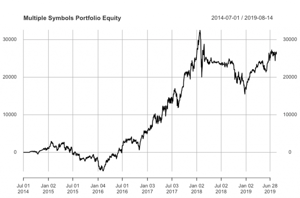
7plot(final_acct$summary$End.Eq, main = "Multiple Symbols Portfolio Equity")
8Multiple Symbols Portfolio Equity Triple EMA Crossover Strategy
Portfolio Statistics
1tStats <- tradeStats(Portfolios = portName, use="trades", inclZeroDays=FALSE)
2
3# Get performance information for each symbol
4
5tab.profit <- tStats %>%
6  select(Net.Trading.PL, Gross.Profits, Gross.Losses, Profit.Factor)
7
8# t: transpose
9
10t(tab.profit)
11
12                    DBC          EEM         EFA          GLD          IWM        IYR
13Net.Trading.PL 266.4998  3713.685370 -629.807645   211.000000  9403.746347 4037.07263
14Gross.Profits  266.4998  4862.953129  125.911927  2752.000000 11603.902733 4354.18955
15Gross.Losses     0.0000 -1149.267759 -755.719572 -2541.000000 -2200.156385 -317.11692
16Profit.Factor        NA     4.231349    0.166612     1.083038     5.274126   13.73055
17                      QQQ       SPY         TLT
18Net.Trading.PL 6569.62866 -708.0645 3222.506379
19Gross.Profits  6890.56991    0.0000 3799.799792
20Gross.Losses   -320.94126 -708.0645 -577.293413
21Profit.Factor    21.46988    0.0000    6.582094
22
23# Average trade profit per symbol
24
25tab.wins <- tStats %>%
26  select(Avg.Trade.PL, Avg.Win.Trade, Avg.Losing.Trade, Avg.WinLoss.Ratio)
27
28(t(tab.wins))
29
30                       DBC         EEM         EFA         GLD         IWM       IYR
31Avg.Trade.PL      266.4998  742.737074 -157.451911   52.750000  3134.58212  807.4145
32Avg.Win.Trade     266.4998 2431.476565   62.955964 2752.000000 11603.90273 1451.3965
33Avg.Losing.Trade       Nan -383.089253 -377.859786 -847.000000 -1100.07819 -158.5585
34Avg.WinLoss.Ratio       NA    6.347024    0.166612    3.249115    10.54825    9.1537
35
36                     QQQ       SPY         TLT
37Avg.Trade.PL      1313.92573 -236.0215  537.084397
38Avg.Win.Trade     1722.64248       Nan  949.949948
39Avg.Losing.Trade  -320.94126 -236.0215 -288.646706
40Avg.WinLoss.Ratio    5.36747       NaN    3.291047
41
42
Cumulative Returns
1# Returns on Equity(ROE) by Symbol
2
3rets <- PortfReturns(Account = acctName)
4
5rownames(rets) <- NULL
6
7# Chart the cumulative returns for all the symbols
8
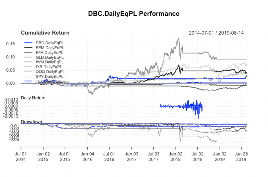
9charts.PerformanceSummary(rets, colorset = bluefocus)
10
11Cumulative Returns by ETF’s Triple EMA Cross Over Strategy
Performance Statistics for Each Symbol
1# Performance Statistics and risk metrics for each symbol
2# Performance : annualized and cumulative returns s
3# Risk metrics : Sharpe and Calmar ratio
4
5tab.perf <- table.Arbitrary(rets,
6                            metrics=c(
7                              "Return.cumulative",
8                              "Return.annualized",
9                              "SharpeRatio.annualized",
10                              "CalmarRatio"),
11                            metricsNames=c(
12                              "Cumulative Return",
13                              "Annualized Return",
14                              "Annualized Sharpe Ratio",
15                              "Calmar Ratio"))
16
17round(tab.perf,5)
18
19                        DBC.DailyEqPL EEM.DailyEqPL EFA.DailyEqPL GLD.DailyEqPL
20Cumulative Return             0.00266       0.03719      -0.00635       0.00190
21Annualized Return             0.00052       0.00716      -0.00124       0.00037
22Annualized Sharpe Ratio       0.24670       0.46053      -0.23570       0.04058
23Calmar Ratio                  0.10078       0.23305      -0.10153       0.01016
24                        IWM.DailyEqPL IYR.DailyEqPL QQQ.DailyEqPL SPY.DailyEqPL
25Cumulative Return             0.09275       0.04061       0.06655      -0.00714
26Annualized Return             0.01748       0.00781       0.01267      -0.00140
27Annualized Sharpe Ratio       0.38301       0.52618       0.57011      -0.24452
28Calmar Ratio                  0.25103       0.38344       0.26922      -0.14163
29                        TLT.DailyEqPL
30Cumulative Return             0.03236
31Annualized Return             0.00624
32Annualized Sharpe Ratio       0.56136
33Calmar Ratio                  0.32163
34
Risk Statistics by Symbol
1# Risk Statistics by Symbol
2
3tab.risk <- table.Arbitrary(rets,
4                            metrics=c(
5                              "StdDev.annualized",
6                              "maxDrawdown",
7                              "VaR",
8                              "ES"),
9                            metricsNames=c(
10                              "Annualized StdDev",
11                              "Max DrawDown",
12                              "Value-at-Risk",
13                              "Conditional VaR"))
14
15round(tab.risk,5)
16
17
18                 DBC.DailyEqPL EEM.DailyEqPL EFA.DailyEqPL GLD.DailyEqPL IWM.DailyEqPL
19Annualized StdDev       0.00210       0.01555       0.00528       0.00914       0.04565
20Max DrawDown            0.00515       0.03072       0.01225       0.03649       0.06962
21Value-at-Risk          -0.00016      -0.00149      -0.00053      -0.00084      -0.00464
22Conditional VaR        -0.00016      -0.00342      -0.00110      -0.00115      -0.01233
23                  IYR.DailyEqPL QQQ.DailyEqPL SPY.DailyEqPL TLT.DailyEqPL
24Annualized StdDev       0.01484       0.02223       0.00572       0.01114
25Max DrawDown            0.02036       0.04705       0.00987       0.01944
26Value-at-Risk          -0.00144      -0.00230      -0.00044      -0.00065
27Conditional VaR        -0.00358      -0.00500      -0.00044      -0.00065
28
The results above show that the symbol IWM has the best performance among all ETFs in the portfolio. The annual returns for IWM was 1,75% and the cumulative return was 9,3%. In the second place comes the QQQ ETF which has an annual return in the whole period of 1,23% and cumulative returns of 6,65%.
The worst performance among the ETF’s in the portfolio was for SPY ETF with an annualized return of -0.14% and a cumulative return of -0,71% in the whole period. Regards, the ETF with the Maximum Drawdown level, we can observe that the IWM ETF has the Maximum Drawdown lever among the rest of the ETF’s with a 7% of Maximum Drawdown.
In terms of Sharpe and Calmar Ratio, the best level of Sharpe Ratio is observed for IWR ETF with a value of 0.38 and Calmar ratio of 0.25. Remember, when we define Calmar Ratio in the risk management section, we point out that this ratio takes into account the Maximum Drawdown level in its calculation. So for a conservative strategy this ratio is fundamental.
Finally the QQQ ETF has the higher Sharpe Ratio with a value of 0.57 which is followed by the TLT ETF with a Sharpe Ratio value of 0.56. Overall, this strategy has positive returns at the end of the period, but is affected by a significant drawdown at the end of 2018. The exit rule of this strategy given by triple EMA cross down is to exit the position when the market reverse.
