Plotting the VIX Index and TED Spread in R

In this lesson, will will look at how to create the two graphs in R. Before you start, it is important to setup your basic environment:

Setup Environment

Open RStudio and ensure that you have the basic setup in place.

• Create a new directory called ‘quantative-trading-strategies-r’ in your computer. We will use this director for all the exercises in this course.
• Set this directory as your working directory using the setwd() command. You can also check the current working directory using the getwd() command in R console.
• Use the command CTRL+L to clear the console (Use this whenever you feel the console is cluttered).
• Create a new R script where we will be writing our R script.
• Install and load the ggplot2 package by typing the following commands in the console:

1#Install ggplot2
2install.packages("ggplot2")
3 
4#Load ggplot2
5library("ggplot2")
6

Plot the TED Spread

In order to plot the TED spread, you can follow the following instructions:

Step 1: Download Data

You can download the data for TED spread from the FRED® Economic Data website.

Get TED data from https://fred.stlouisfed.org/series/TEDRATE

For convenience, we have also provided the data files below.

You can download the data file and save it in your working directory.

Step 2: Load the data in your R Environment

To read a csv with R, the best way to do it is with the command read.csv.

1ted <- read.csv("TEDRATE.csv",stringsAsFactors = FALSE)
2

Step 3: Transform Data

The read.csv function interpret both columns as factors columns, so we need to change to the appropriate columns data types.

We will convert character columns to numeric and date columns, and remove NA values with complete.cases.

The complete.cases function returns a logical vector specifying which observations/rows have no missing values across the entire sequence.

1ted$TEDRATE <- as.numeric(ted$TEDRATE)
2ted$DATE <- as.Date(ted$DATE)
3ted <- ted[complete.cases(ted),]
4

Finally, we have ‘ted’ as a dataframe containing our prepared data.

Step 4: Plot the Graph

Now, we can use ggplot2 library to plot the graph.

1ggplot(ted, aes(DATE, TEDRATE)) + geom_line(color = "red") + xlab("") + ylab("Daily Prices")+ggtitle("TED Spread")
2

The complete script for creating the TED spread is provided below:

1# Get TED data from https://fred.stlouisfed.org/series/TEDRATE
2# Load the data using read.csv
3
4ted <- read.csv("TEDRATE.csv",stringsAsFactors = FALSE)
5
6# The read.csv function interpret both columns as factors columns, so we need to change
7# to the appropriate columns data types. Convert character columns to numeric and date
8# columns, and remove NA values with complete.cases
9
10ted$TEDRATE <- as.numeric(ted$TEDRATE)
11ted$DATE <- as.Date(ted$DATE)
12ted <- ted[complete.cases(ted),]
13
14# View the data
15ted
16
17# Plot the graph
18
19ggplot(ted, aes(DATE, TEDRATE)) + geom_line(color = "red") + xlab("") + ylab("Daily Prices")+
20  ggtitle("TED Spread")
21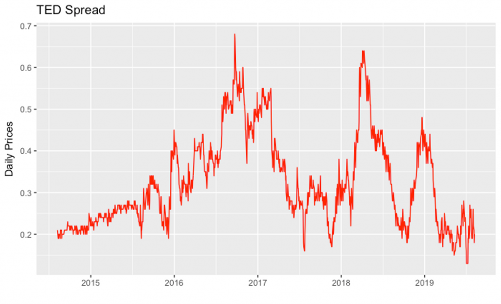

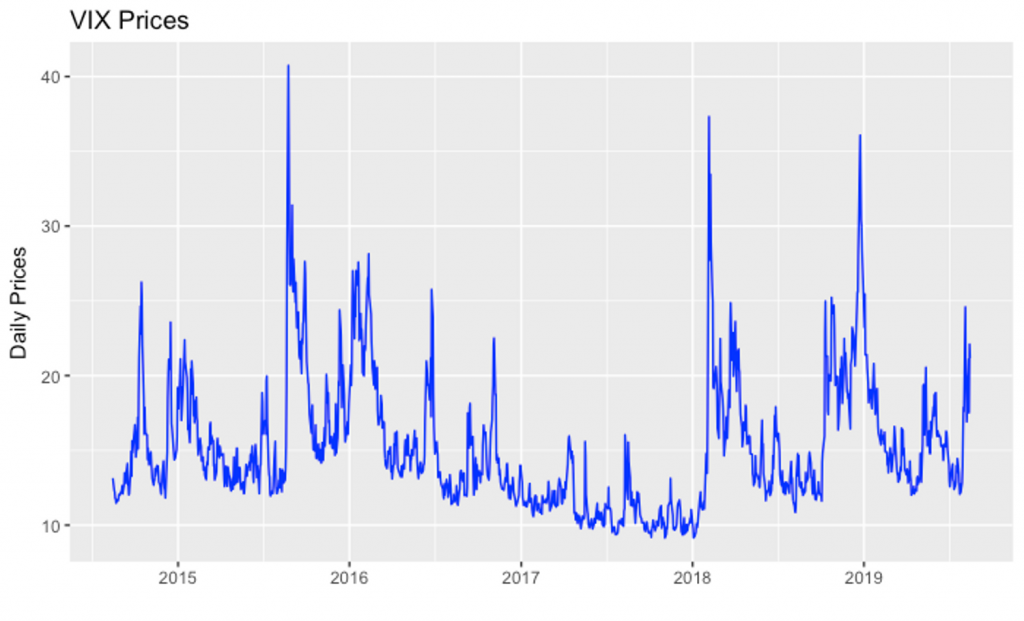
Plot the VIX Index

You can follow the exact same steps above to plot the VIX volatility index. The complete script for it is provided below:

1# Get VIX data from https://fred.stlouisfed.org/series/VIXCLS
2# Load the data using read.csv
3
4VIX <- read.csv("VIXCLS.csv",stringsAsFactors = FALSE)
5
6# Convert character columns to numeric and date columns, and 
7# remove NA values # with complete.cases
8
9VIX$VIXCLS <- as.numeric(VIX$VIXCLS)
10VIX$DATE <- as.Date(VIX$DATE)
11VIX <- VIX[complete.cases(VIX),]
12
13# View the data
14VIX
15
16# Plot the graph
17
18ggplot(VIX, aes(DATE, VIXCLS)) + geom_line(color = "blue") + xlab("") + ylab("Daily Prices")+
19  ggtitle("VIX Prices")
20