Measuring Overall ETFs Performance
We will now plot a graph to show the accumulated returns of the ETFs over a period of time. We can do so by following the following steps:
- Build a dataframe with the 4 ETFs prices and a date column. Calculate daily returns and cumulative returns. The cumsum() function returns the cumulative sums (i.e. the sum of all values up to a certain position of a vector).
- Change the format of the data from wide shape to long shape with the gather() function from dplyr package.
- Use ggplot2 to graph the ETFs performance in the whole period.
Step 1: Build a dataframe with the 4 ETFs prices and a date column. Calculate daily returns and cumulative returns.
1# Make the cumRets dataframe with the cumulative returns for each of the ETFs using cumsum() function
2# The dailyReturn is a built in function from quantmod to get the daily returns.
3
4cumRets <- data.frame(date = index(SPY),
5                cumsum(dailyReturn(SPY) * 100),
6                 cumsum(dailyReturn(IVV) * 100),
7                 cumsum(dailyReturn(QQQ)* 100),
8                 cumsum(dailyReturn(IWF))* 100)
9
10# Add new names to the columns of cumRets dataframe
11
12colnames(cumRets)[-1] <- etfs
13
14head(cumRets,10)
15
16         date     SPY     IVV     QQQ     IWF
171  2014-02-03 -2.1352 -2.1233 -2.1136 -2.2921
182  2014-02-04 -1.4347 -1.4382 -1.3780 -1.3709
193  2014-02-05 -1.5602 -1.5686 -1.6371 -1.6752
204  2014-02-06 -0.2414 -0.2345 -0.3619 -0.2958
215  2014-02-07  0.9981  1.0709  1.4220  1.1491
226  2014-02-10  1.1818  1.2092  1.9947  1.4221
237  2014-02-11  2.2762  2.3137  3.1337  2.4401
248  2014-02-12  2.3256  2.3957  3.3251  2.6393
259  2014-02-13  2.8419  2.8814  4.0669  3.3410
2610 2014-02-14  3.3938  3.4137  4.2677  3.5616
27
Step 2: Change the format of the data from wide shape to long shape with the gather function from dplyr package.
The data is currently wide-shaped because each date’s data is wide. For better analysis, We want the data to be long, where each date of data is in a separate observation.
1# Make a tidy dataset called longCumRets which group the returns of each ETF in the same column.
2# The second and third parameter of the gather function are the new columns names in the tidy dataset.
3
4# Note: You need to install the tidyr package to use the gather function. Use install.packages('tidyr') for installing and library(tidyr) to load it.
5
6longCumRets <- gather(cumRets,symbol,cumReturns,etfs)
7
8head(longCumRets,10)
9
10         date symbol cumReturns
111  2014-02-03    SPY    -2.1352
122  2014-02-04    SPY    -1.4347
133  2014-02-05    SPY    -1.5602
144  2014-02-06    SPY    -0.2414
155  2014-02-07    SPY     0.9981
166  2014-02-10    SPY     1.1818
177  2014-02-11    SPY     2.2762
188  2014-02-12    SPY     2.3256
199  2014-02-13    SPY     2.8419
2010 2014-02-14    SPY     3.3938
21
Step 3: Use ggplot2 to graph the ETFs performance in the whole period.
1# Plot the performance of the ETF's indexes
2
3ggplot(longCumRets, aes(x=date,y=cumReturns,color = symbol))  + geom_line()+ ggtitle("ETF’s Accumulated Returns")
4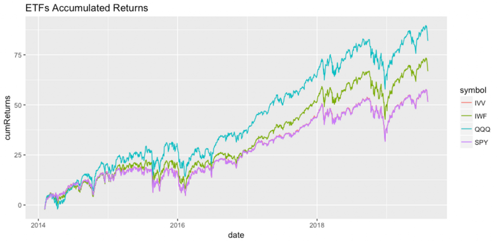
As we can observe in the graph, all ETFs are correlated, which means that they are affected by similar drivers. QQQ has the greatest performance in the whole period while SPY and IVV have the lowest performance. At the end of 2018 a big drawdown has affected all ETFs performance.
A note about reshaping data:
There are times when our data is considered unstacked and a common attribute of concern is spread out across columns. To reformat the data such that these common attributes are gathered together as a single variable, the gather() function will take multiple columns and collapse them into key-value pairs, duplicating all other columns as needed.
Measuring Overall ETFs Performance - Yearly Breakdown
To go deeper in analyzing ETFs performance during the period, we will make a breakdown about ETF performance by year. With this picture we can gain an insight into which ETF has the greater and poor performance by year. This can be achieved by following the following steps:
- Step 1: Transform the returns dataframe from wide to long creating the longrets dataframe. With this shape, we would have two new columns that are symbol and returns, which store the daily returns for each symbol in long format.
- Step 2: Make a new column in longrets with only the year from the index of returns.
- Step 3: Calculate the mean of returns for each group, where the group is composed of a particular symbol-year.
1# Transform the returns dataframe from wide to long creating the longrets dataframe.
2
3longrets <- gather(returns,symbol,returns,etfs)
4
5head(longrets)
6
7  symbol returns
81    SPY -2.1352
92    SPY  0.7005
103    SPY -0.1254
114    SPY  1.3187
125    SPY  1.2396
136    SPY  0.1837
14
15
16# Take only the years from the index names of returns that have the dates
17
18longrets$year <- substr(rownames(returns),1,4)
19
20head(longrets)
21
22  symbol returns year
231    SPY -2.1352 2014
242    SPY  0.7005 2014
253    SPY -0.1254 2014
264    SPY  1.3187 2014
275    SPY  1.2396 2014
286    SPY  0.1837 2014
29
30# The aggregate function can split a data frame columns by groups and then
31# apply a function to these groups. In our case the column that we are
32# interested to split is the returns column and the groups are symbol and year.
33# Finally we will apply the mean function to each of these groups.
34
35groupedReturns <- aggregate(longrets$returns, list(symbol=longrets$symbol,year=longrets$year), mean)
36
37groupedReturns
38
39  symbol year            x
401     IVV 2014  0.065175325
412     IWF 2014  0.062363203
423     QQQ 2014  0.082309524
434     SPY 2014  0.064810823
445     IVV 2015  0.001005556
456     IWF 2015  0.020585714
467     QQQ 2015  0.038149603
478     SPY 2015  0.001565079
489     IVV 2016  0.040590079
4910    IWF 2016  0.024551190
5011    QQQ 2016  0.028030159
5112    SPY 2016  0.039951587
5213    IVV 2017  0.071888048
5314    IWF 2017  0.100740637
5415    QQQ 2017  0.111167729
5516    SPY 2017  0.071519124
5617    IVV 2018 -0.020522311
5718    IWF 2018 -0.003539841
5819    QQQ 2018  0.006568924
5920    SPY 2018 -0.020306375
6021    IVV 2019  0.088256376
6122    IWF 2019  0.111604027
6223    QQQ 2019  0.112140940
6324    SPY 2019  0.088615436
64
65
The groupedReturns dataframe provides useful insights about the mean returns of each ETF by year. We can see that the best symbol-year was QQQ 2019 with mean returns of 11%, while the poor symbol-year performance was IVV 2018 with a mean return of -2%. It is very appealing to show these insights graphically.
1annReturnBars <- ggplot(groupedReturns,aes(x=symbol,y=x)) +
2  geom_bar(stat="identity",aes(fill=symbol))+
3  facet_wrap(~year,ncol=2) +
4  theme(legend.position = "right") + ggtitle("ETF mean returns by Year")
5
6annReturnBars
7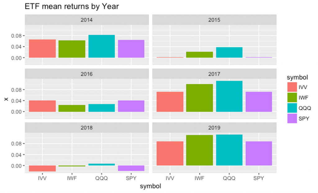
In this bar plot chart we can observe that the QQQ ETF has the highest performance in all years, except for 2016 where the most performant was IVV ETF. Also we can observe that 2018 was the worst year of the period, where only QQQ has slightly positive returns. On the other hand, 2017 were a good year for all ETFs, and up to this moment 2019 is a good year too.
In the next section, we would start with the quantstrat package that provides an infrastructure to build, backtest and analyze trading strategies.
