Expected Loss, Unexpected Loss, and Loss Distribution
While the terms expected loss and unexpected loss are commonly used in risk management, it is important to have a clear understanding of what they actually mean.
While the terms expected loss and unexpected loss are commonly used in risk management, it is important to have a clear understanding of what they actually mean.
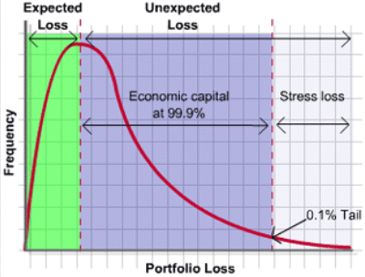
In general, expected loss as the name suggests is the expected loss from a loan exposure. On the other hand unexpected loss is the loss that exceeds the expectations.
Expected Loss In statistical terms, the expected loss is the average credit loss that we would expect from an exposure or a portfolio over a given period of time.
The expected loss is measured using the following formula:
Portfolio Expected Loss: The total expected loss of a portfolio will simply be the summation of expected losses of individual assets. This is because the mean of the sum is the same as the sum of the mean.
Since the expected loss is what a business expects to lose in a year, the business will generally have budget for it and the losses can be borne as a part of the normal operating cash flows.
Unexpected Loss The unexpected loss is the average total loss over and above the mean loss. It is calculated as a standard deviation from the mean at a certain confidence level at a certain confidence level. It is also referred to as Credit VaR.
A business will safeguard itself from unexpected losses by allocating capital.
Unlike expected loss, the expected loss of a portfolio is not calculated by adding the unexpected loss of individual assets. This is because unless there is perfect correlation, the standard deviation of sum will not be the same as the sum of standard deviation.
The unexpected loss of a portfolio at a 99% confidence level will be expressed as follows:
UL99% = D99% - EL
Where D99% represents the 99% Var Quantile.
If the 99% VaR level is $200m and the expected portfolio loss is $50, then the unexpected loss will be $150m.
The unexpected loss of a portfolio will be expressed as follows:
Apart from the expected and unexpected losses, there are also catastrophic losses, which are covered by insurance.
The Credit Loss Distribution The following diagram shows the credit loss distribution.

Characteristics of Credit Loss Distribution
The credit losses distribution has three key characteristics:
- It is not symmetrical. There is a limited upside because the best scenario is when there is no loss. However, there is extremely large downside, that is, the losses can be huge.
- It is highly skewed. The distribution is more concentrated toward small losses, with very few chances of large losses.
- The distribution has heavy tail, i.e., the probability of large losses reduces very slowly.


