In R, we can create a line plot using the same plot() function by adding a plot type of "l". This will plot the (x,y) paired observations and connect them with lines.

plot(x,y,type="l")

Let's generate our own data for this lesson. We will use the rnorm() function to generate a set of 100 random numbers that follow a normal distribution. These random numbers will be plotted on y-axis. x-axis will be a sequence of numbers from 1 to 100.

> x <- c(1:100)
> rand_data <- rnorm(100, mean = 0)
> data <- data.frame(x, rand_data)
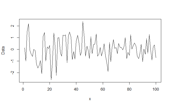
> plot(data$x, data$rand_data, type = "l", xlab="x", ylab = "Data")

The resulting line plot is displayed below:

Line Type

You can change the appearance of the line by using the lty parameter.

• lty="solid" or lty=1 (default)
• lty="dashed" or lty=2
• lty="dotted" or lty=3
• lty="dotdash" or lty=4
• lty="longdash" or lty=5
• lty="twodash" or lty=6
• lty="blank" or lty=0

Line Width

The line width can be changed using the lwd parameter. The default width is 1. So, you can plot a thicker line using a higher number.

Line Color

The line color can be changed using the col parameter.

Below we replot the line plot with a dotted line, thickness of 2, and in orange color.

> plot(data$x, data$rand_data, type = "l", xlab="x", ylab = "Data",lty=3,lwd=2,col="orange")

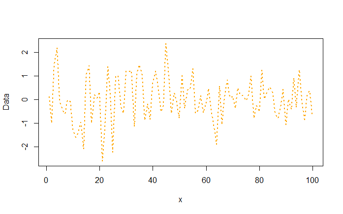
Line Chart

Exercise

We know that numerical data generally conforms to a normal probability distribution characterized by a bell curve. In this exercise you are asked to create a bell curve using the normal data.

• Use the rnorm() function to generate random numbers that follow a normal distribution (mean 0 and standard deviation of 1). Generate upto 5000 numbers. Store these numbers in a variable x.
• Plot the density of these random numbers using plot(density(x)) This will plot the bell curve.
• Try different values for mean and standard deviation and observe how the graph changes.

Note: You can also compute the Gaussian density using the dnorm() function, for example dnorm(x, mean = 0, sd = 1).