Calculating VaR Using Historical Simulation
The fundamental assumption of the Historical Simulations methodology is that you base your results on the past performance of your portfolio and make the assumption that the past is a good indicator of the near-future. The below algorithm illustrates the straightforwardness of this methodology. It is called Full Valuation because we will re-price the asset or the portfolio after every run. This differs from a Local Valuation method in which we only use the information about the initial price and the exposure at the origin to deduce VaR.
The fundamental assumption of the Historical Simulations methodology is that you base your results on the past performance of your portfolio and make the assumption that the past is a good indicator of the near-future.
The below algorithm illustrates the straightforwardness of this methodology. It is called Full Valuation because we will re-price the asset or the portfolio after every run. This differs from a Local Valuation method in which we only use the information about the initial price and the exposure at the origin to deduce VaR.
Step 1 – Calculate the returns (or price changes) of all the assets in the portfolio between each time interval.
The first step lies in setting the time interval and then calculating the returns of each asset between two successive periods of time.
Generally, we use a daily horizon to calculate the returns, but we could use monthly returns if we were to compute the VaR of a portfolio invested in alternative investments (Hedge Funds, Private Equity, Venture Capital and Real Estate) where the reporting period is either monthly or quarterly. Historical Simulations VaR requires a long history of returns in order to get a meaningful VaR. Indeed, computing a VaR on a portfolio of Hedge Funds with only a year of return history will not provide a good VaR estimate.
Step 2 – Apply the price changes calculated to the current mark-to-market value of the assets and re-value your portfolio.
Once we have calculated the returns of all the assets from today back to the first day of the period of time that is being considered – let us assume one year comprised of 265 days – we now consider that these returns may occur tomorrow with the same likelihood. For instance, we start by looking at the returns of every asset yesterday and apply these returns to the value of these assets today. That gives us new values for all these assets and consequently a new value of the portfolio. Then, we go back in time by one more time interval to two days ago. We take the returns that have been calculated for every asset on that day and assume that those returns may occur tomorrow with the same likelihood as the returns that occurred yesterday. We re-value every asset with these new price changes and then the portfolio itself. And we continue until we have reached the beginning of the period. In this example, we will have had 264 simulations.
Step 3 – Sort the series of the portfolio-simulated P&L from the lowest to the highest value.
After applying these price changes to the assets 264 times, we end up with 264 simulated values for the portfolio and thus P&Ls. Since VaR calculates the worst expected loss over a given horizon at a given confidence level under normal market conditions, we need to sort these 264 values from the lowest to the highest as VaR focuses on the tail of the distribution.
Step 4 – Read the simulated value that corresponds to the desired confidence level.
The last step is to determine the confidence level we are interested in – let us choose 99% for this example. One can read the corresponding value in the series of the sorted simulated P&Ls of the portfolio at the desired confidence level and then take it away from the mean of the series of simulated P&Ls. In other words, the VaR at 99% confidence level is the mean of the simulated P&Ls minus the 1% lowest value in the series of the simulated values. This can be formulated as follows:
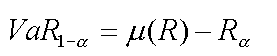
Where:
- VaR (1 - ) is the estimated VaR at the confidence level 100 × (1 - )%.
- (R) is the mean of the series of simulated returns or P&Ls of the portfolio
- R is the worst return of the series of simulated P&Ls of the portfolio or, in other words, the return of the series of simulated P&Ls that corresponds to the level of significance
Need for Interpolation We may need to proceed to some interpolation since there will be no chance to get a value at 99% in our example. Indeed, if we use 265 days, each return calculated at every time interval will have a weight of 1/264 = 0.00379. If we want to look at the value that has a cumulative weight of 99%, we will see that there is no value that matches exactly 1% (since we have divided the series into 264 time intervals and not a multiple of 100). Considering that there is very little chance that the tail of the empirical distribution is linear, proceeding to a linear interpolation to get the 99% VaR between the two successive time intervals that surround the 99th percentile will result in an estimation of the actual VaR. This would be a pity considering we did all that we could to use the empirical distribution of returns, wouldn’t it? Nevertheless, even a linear interpolation may give you a good estimate of your VaR. For those who are more eager to obtain the exact VaR, the Extreme Value Theory (EVT) could be the right tool for you. We will explain in another article how to use EVT when computing VaR. It is rather mathematically demanding and would require us to spend more time to explain this method.
