In the binomial option pricing model, the value of an option at expiration time is represented by the present value of the future payoffs from owning the option. The main principle of the binomial model is that the option price pattern is related to the stock price pattern. In this post, we will learn about how to build binomial option pricing model in R.

First we will value an option with a single period until expiration.  The price of a call in the frame of the single period binomial model can be represented using the following equation that represents a synthetic European call option:

ct = N * St - Bt

N=Number of Shares in the Portfolio

St = Stock price at t

Bt\=Short position in a risk-free bond

Using this equation we can replicate the value of a call at expiration by owning a portfolio with N number of shares for a stock with price St  and with an amount borrowed B at the risk-free rate. In a single period if the stock price St goes up, the call option price will increase, and if the stock price St decreases, the call option would fall.

The value of the call can be expressed in terms of the likelihood of price movements in the underlying asset on the next period. When the stock price goes up, the call pays CU  at expiration, and when the stock price goes down the call pays CD. This led to the following equation:

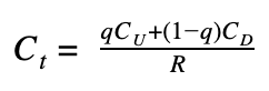
Where  q is the probability that the stock goes up and (1-q) is the probability that the stock goes down and R is the risk free rate, at which the option payoff is discounted in each period. The representation of the likelihood of an increase or decrease on the stock price can be constructed using the stock price volatility ?.

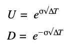
Cox, Ross, and Rubinstein (1979) proposed the following formulas of U and D:

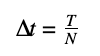
T represents the time. If T = 1 means that T is one year, and if T=0.25 represent 3 months. The number of periods we simulate the stock price is N. Then the amount of time represented by each period is:

Having the values of the volatility ?, the time of expiration, and the number of periods N, we can simulate the stock price in N periods with the following function called build_stock_tree:

build_stock_tree <- function(S, sigma, delta_t, N) {
  tree = matrix(0, nrow=N+1, ncol=N+1)
  U = exp(sigma*sqrt(delta_t))
  D = exp(-sigma*sqrt(delta_t))
  for (i in 1:(N+1)) {
    for (j in 1:i) {
      tree[i, j] = S * U^(j-1) * D^((i-1)-(j-1))
    }  }
  return(tree)
}

The above code first initializes a matrix which is called tree with N +1 number of rows and N+1 number of columns. Then, it defines U and D (the different paths of the stock price) with the formulas that we set above and afterwards, the for loop would fill the tree matrix with the valuation price in each of the leaf nodes.

If we have a stock price of USD 80, with a volatility of 0.1 and 2 periods we can build a tree with the function build_stock_tree and simulate the stock price. The results are the following:

firstExample <- build_stock_tree(S=80, sigma=0.1, delta_t=1/2, N=2)

         [,1]     [,2]     [,3]
[1,] 80.00000  0.00000  0.00000
[2,] 74.53851 85.86165  0.00000
[3,] 69.44988 80.00000 92.15279

Each time we change N, ∆t will change too. In case N=4, ∆t=1/4 and the new stock tree is:

secondExample <- build_stock_tree(S=80, sigma=0.1, delta_t=1/4, N=4)

         [,1]     [,2]     [,3]     [,4]     [,5]
[1,] 80.00000  0.00000  0.00000  0.00000  0.00000
[2,] 76.09835 84.10169  0.00000  0.00000  0.00000
[3,] 72.38699 80.00000 88.41367  0.00000  0.00000
[4,] 68.85664 76.09835 84.10169 92.94674  0.00000
[5,] 65.49846 72.38699 80.00000 88.41367 97.71222

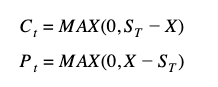
Next step is to get the binomial tree for options pricing. A call option value at expiration is given by the MAX(S-K,0), where K is the strike price of the call option. In our second example, if the strike price K is USD 85, the intrinsic value of the option related to the different stock paths would be:

K <- 85
IntrinsecValue <- secondExample[5,] – K
IntrinsecValue[IntrinsecValue<0] <- 0

[1]  0.000000  0.000000  0.000000  3.413673 12.712221

The first three values would be zero because the option is not worthless as the Stock price is lower than the strike price. Finally we need a function to discount the options prices at the different periods and which incorporate the likelihood of an increase or decrease in the stock price. This is given by the q parameter q that is formulated on different Financials books as:

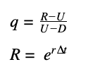
This formula of can be expressed in the following function q_prob:

q_prob <- function(r, delta_t, sigma) {
  u = exp(sigma*sqrt(delta_t))
  d = exp(-sigma*sqrt(delta_t))
    return((exp(r*delta_t) - d)/(u-d))
}

Finally, the above functions can be combined and create a complete function to value options in each leaf node of the tree. The following function called value_binomial_option would do that job.

value_binomial_option <- function(tree, sigma, delta_t, r, X, type) {
  q = q_prob(r, delta_t, sigma)
  option_tree = matrix(0, nrow=nrow(tree), ncol=ncol(tree))
  if(type == 'put') {
    option_tree[nrow(option_tree),] = pmax(X - tree[nrow(tree),], 0)
  } else {  option_tree[nrow(option_tree),] = pmax(tree[nrow(tree),] - X, 0)
  }
  for (i in (nrow(tree)-1):1) {
    for(j in 1:i) {
     option_tree[i,j]=((1-q)*option_tree[i+1,j] +        q*option_tree[i+1,j+1])/exp(r*delta_t)
    }
  }
  return(option_tree)
}

The value_binomial_option function receives 7 inputs that are: tree, sigma, delta_t, r, X, and type. The tree parameter is the output of the build_stock_tree function that was described previously. Sigma is the volatility of the stock price, delta_t is the time period in which the option expires, r is the risk free interest rate, X is the strike price of the option at expiration and  type should be ‘put’ for put options valuation and ‘call’ for call options valuation.

This function has three main steps. The first step consists of calculating q given the values of r, delta_t and sigma. Then the function initializes the tree matrix with the correct dimensions.  For this purpose, we define the option_tree structure as a matrix with the same dimensions of the stock tree. 

Secondly, we calculate the intrinsic value of the options at expiration time.  For this task, the last row of the option_tree matrix is filled with the max value between 0 and the difference of the Strike price and the Stock Price at expiration if the option type is ‘put’, or the max value between 0 and the difference between the Stock Price and the Strike price if the type is ‘call’.

The third part consists of a for loop that would fill the option_tree structure in backward direction starting with the values from the last row (that were calculated and assigned in the previous step) of the matrix.

option_tree[i, j] = ((1-q)*option_tree[i+1,j] +q*option_tree[i+1,j+1])/exp(r*delta_t)

In this line, i refer to a specific row number of the tree and j refers to a specific column number. As we stated above the loop has backward direction and gets the values from the last row which are the intrinsic values of the options at expiration. For each intersection of the i row’s and j column’s  is calculated the option prices at the current period given  the probability of an up movement in the price(q) and the probability of a down movement in the  price(1-q) on the next period divided by R which is the rate of discount. 

The binomial_option function would join all the functions that we have described and will return a tree with the values of the option at the different periods. These are the payoffs of the option on the different periods during the option life.

binomial_option <- function(type, sigma, T, r, X, S, N) {
  q <- q_prob(r=r, delta_t=T/N, sigma=sigma)
  tree <- build_stock_tree(S=S, sigma=sigma, delta_t=T/N, N=N)
  option <- value_binomial_option(tree, sigma=sigma, delta_t=T/N, r=r, X=X, type=type)
  return(list(q=q, stock=tree, option=option, price=option[1,1]))
}

The binomial_option function runs the three functions that we described which are q_prob, build_stock_tree and value_binomial_option, and returns a list with the values of  q, the stock tree, the option tree, and the option price. 

In order to run the binomial function, we need to insert the correct inputs. If we want to value a call option with X = 100, S = 110, N=5, sigma = 0.15, r=01 

results <- binomial_option(type='call', sigma=0.15, T=1, r=0.1, X=100, S=110, N=5)

And the results of this is a list structure with 4 items (q, stock tree, option tree and the option value). We can retrieve each element of the result list with ‘$’ operator.

results$q

[1] 0.6336948

results$stock

         [,1]      [,2]     [,3]     [,4]     [,5]     [,6]
[1,] 110.00000   0.00000   0.0000   0.0000   0.0000   0.0000
[2,] 102.86303 117.63215   0.0000   0.0000   0.0000   0.0000
[3,]  96.18912 110.00000 125.7938   0.0000   0.0000   0.0000
[4,]  89.94823 102.86303 117.6322 134.5218   0.0000   0.0000
[5,]  84.11225  96.18912 110.0000 125.7938 143.8554   0.0000
[6,]  78.65492  89.94823 102.8630 117.6322 134.5218 153.8365

results$option

         [,1]      [,2]      [,3]     [,4]     [,5]     [,6]
[1,] 20.162476  0.000000  0.000000  0.00000  0.00000  0.00000
[2,] 12.062180 25.487578  0.000000  0.00000  0.00000  0.00000
[3,]  5.415450 16.288826 31.617395  0.00000  0.00000  0.00000
[4,]  1.104625  8.079946 21.553209 38.44289  0.00000  0.00000
[5,]  0.000000  1.778364 11.980133 27.77398 45.83552  0.00000
[6,]  0.000000  0.000000  2.863033 17.63215 34.52183 53.83653

results$price

[1] 20.16248

To conclude, we can use this model to show the relationship between options and Strikes prices. We can create an array of Strike prices and wrap the binomial_option function in another function and vary the Strike parameter to get an array of option prices for different Strikes at expiration. We would define the option_price_vary_function that wraps the binomial_function and allows different values to the strike parameter.  

# Define an array with strike prices between 80 and 120

strikes <- seq(80, 120)

option_price_vary_function <- function(strike) { option = binomial_option(type='call', sigma=0.15, T=1, r=0, X=strike, S=110, N=5)
  return(option$price)
}

# Use the sapply command to pass each value of the strikes array into the option_price_vary_strike function:

values <- sapply(strikes, option_price_vary_period)

# Create a data frame with the Strikes prices and the option prices (values) from above

data <- as.data.frame(list(strikes=strikes, values=values)) 

head(data)

  strikes   values
1      80 30.04957
2      81 29.08642
3      82 28.12327
4      83 27.16013
5      84 26.19698
6      85 25.23383

Lastly we use the ggplot package to plot the relationship between option prices and strikes values.

ggplot(data=data) + geom_line(aes(x=strikes, y=values)) + labs(title="Call Value", x="Strikes", y="Value") +   geom_vline(xintercept = 100, linetype="dotted",  color = "red", size=1.5)

Call Prices vs Strike Prices 

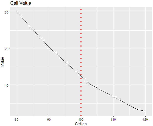
This graph shows the relationship between option prices and strikes prices. Having a stock price of USD100 at expiration, options with strikes prices higher than USD100 have lower values because they are out-of-the-money. On the other hand options that are in-the-money (left side of the red line), have higher values.