How to Build Efficient Frontier in Excel

As we know, an efficient frontier represents the set of efficient portfolios that will give the highest return at each level of risk or the lowest risk for each level of return. A portfolio is efficient if there is no alternative with:

• Higher expected return with same level of risk
• Same expected return with lower level of risk
• Higher expected return for lower level of risk

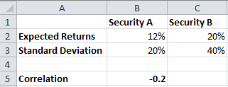
Let’s take a portfolio of two assets and see how we can build the efficient frontier in excel. Let’s say we have two securities, A and B, with the following risk-return data.

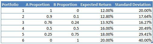
We can combine these two assets to form a portfolio. In the portfolio, we can combine the two assets with different weights for each asset to create an infinite number of portfolios having different risk-return profiles. For example, if we take 50% of each asset, the expected return and risk of the portfolio will be as follows:

E(R) = 0.50*12% + 0.50*20% = 16%

σ = Sqrt(0.20^2*0.5^2+0.40^2*0.5^2+2*(-0.2)*0.5*0.5*0.2*0.4) = 20.49%

The following table shows the risk-return profile for different portfolios created by combining the two assets in different weights.

The risk and return of these portfolios can be plotted on the XY scatter graph with risk on x-axis and return on Y axis. The graph looks as follows and is called the efficient frontier.

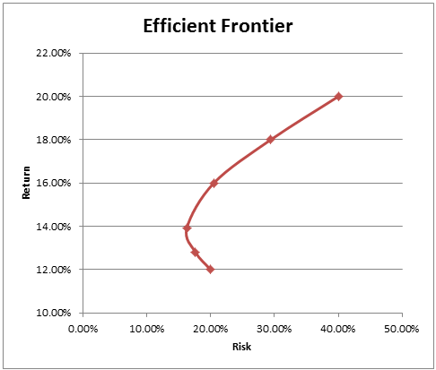
Note that this graph was created with just two assets in the portfolio. The efficient frontier can be created using multiple assets. This frontier represents all the feasible portfolio combinations that one can create. There is also a minimum variance portfolio (MVP) for which there is minimum risk. An investor will not want to purchase a portfolio below the MVP. The curve bends backwards which indicates the benefits of diversification due to negative correlation.