Financial Modelling: Writing Formulas in Excel
In have already looked at the excel keyboard shortcuts that you must know to become productive with excel. The next thing we will look at is how to write effective formulas.
This is an important topic and I believe the quality of your financial model will depend on how well you write the formulas. There are three reasons why it is very important to think and plan about how you write each formula:
- Your financial model is probably going to be used by others in your organizations and they should be able to make use of what you’ve created.
- You will most likely be using the financial model for a long period and when you use it, you may have to tweak it. You shouldn’t have to make major changes to the formulas every time you want to extend the model. For example, if your model contained financial projects upto 2018, and the next year you want to extend it upto 2020, it should simply be a matter of copying and pasting the formulas to the new cells/rows rather than having to make changes to the formula.
- The formula should be simple and short so that you yourself can make sense of it when you try to read it after a long gap.
Let’s take a simple example of calculating the present value of a series of cash flows. Let’s say that you are making an investment that will pay you $1,000 at the end of each year for the next five years. If you had placed the money in a bank deposit, you would have received an interest of 12% p.a. Let’s say that this is the interest that your investment also pays. Based on this information, we can calculate the value of this investment today. Let’s see how.
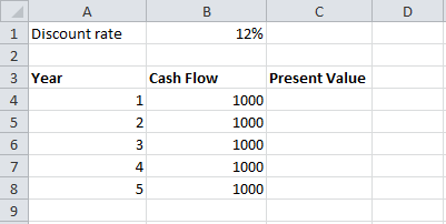
The below screenshot shows the information that we have:

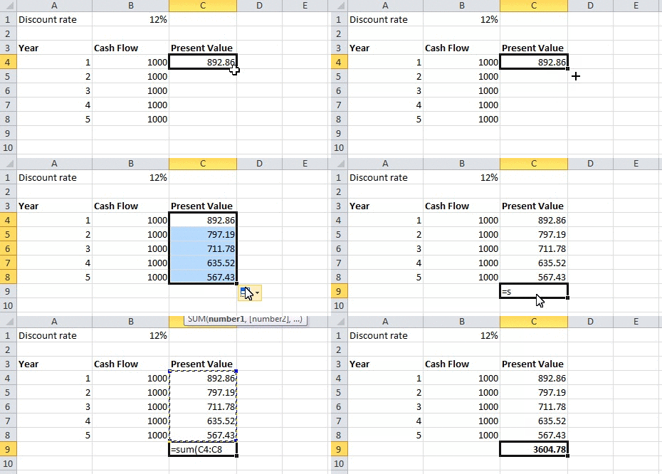
We can calculate the value of this investment by discounting the cash flows with the discount rate. Alternatively we can also calculate it using Excel’s built-in PV function. The following screenshot shows the formula using the first method:

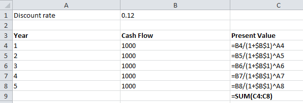
Let’s dissect the formula to understand what we’ve done. I press CTRL + ` to view all formulas in the spreadsheet as shown below:

Notice that I built the formula just for the first cash flow in cell C4. While building the formula, I refer to other cells for their values instead of entering the values directly in the formula. There are two types of cell referencing: relative referencing and absolute referencing. By default, all referencing is relative referencing. So, I refer to the first cash flow in cell B4. ‘=B4’ has relative referencing. If I drag the formula downwards or to the right, the cell reference will automatically change. For example, if I move to row 5, but continue to be in the same column, the formula will change to B5. Similarly, if I move to Column C, but continue to be in the same row, the formula will change to C4. In our case, our cash flows are presented in rows B4:B8. Similarly, we have no problem with year referencing also. However, referencing the discount rate poses a challenge because it’s a fixed value present in cell B1. If we just type ‘B1’ in our formula, it’s not going to work when we drag/copy the formula to other cells. As soon as we copy the formula to the next cell below, B1 is going to become B2. We don’t want that to happen. For this reason, we will make use of absolute referencing. Notice that for discount rate, we’ve entered cell reference as $B$1.
The dollar sign tells Excel to make the referencing absolute. The dollar sign before the column reference makes the column absolute, while the dollar sign before the row reference makes the row absolute. In our case, since our data changes in different rows, we could also have written it as B$1 and it would have worked just fine.
Also notice the use of ‘^’ symbol to represent the power.
Once we have perfected the formula in one cell, we can simply drag it down to fill the rest of the cells with the formula.
Once we have the present value of each cash flow, we can use the SUM function to sum it up and get the present value of cash flows.
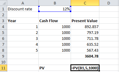
The alternative method is to just use the PV function present in excel. This function takes three parameters, namely, the interest rate, number of periods, and the value of each cash flow.

The PV function can be used only when all the cash flows are same. If they were not, we could use the NPV function which is more suitable for uneven cash flows.
In the above example, I’ve summed up the cash flows right below the cash flows. This is not always a good idea. In a good financial model, you would have to consider the possibility of extending the cash flows beyond five years and then you would have to shift the position of the formula. Instead, a better choice would be to calculate the final value in a designated area on the top of the spreadsheet. We will see this in other examples in the upcoming lessons.


